7  From Features to a Class

Take the features built in Ch 5 and Ch 6 and turn them into a class label per epoch. Compare three approaches: argmax on CCA scores (no training), LDA on spectral features (trained), and the CH11 baseline (already in the data). The goal is to make the fusion of feature engineering and modelling for SSVEP explicit.

7.1 Setup

Same pipeline as the previous chapters, condensed. We end with three things on hand: epochs (the trial tensor), labels (the trigger truth), and y itself (so we can also evaluate the CH11 baseline).

from pathlib import Path
import numpy as np
import scipy.io
import matplotlib.pyplot as plt
from scipy.signal import welch, butter, filtfilt, iirnotch
from sklearn.cross_decomposition import CCA
from sklearn.discriminant_analysis import LinearDiscriminantAnalysis
from sklearn.model_selection import LeaveOneOut

DATA_DIR = Path("data")
STIM_FREQS = [9, 10, 12, 15]
HARMONICS = [1, 2]
N_HARMONICS = 2
NPERSEG = 512
SUB_BANDS = [(6, 14), (14, 22), (22, 30), (30, 40)]

mat = scipy.io.loadmat(DATA_DIR / "subject_2_fvep_led_training_2.mat")
fs = int(mat["fs"][0, 0])
y = mat["y"]


def make_filters(fs, low=5.0, high=40.0, line=50.0, order=4, notch_q=30):
    bp_b, bp_a = butter(order, [low, high], btype="band", fs=fs)
    n_b, n_a = iirnotch(line, notch_q, fs=fs)
    return (bp_b, bp_a), (n_b, n_a)


def apply_filters(x, bp, notch):
    return filtfilt(*notch, filtfilt(*bp, x))


def find_trials(y):
    ch10 = y[9].astype(int)
    active = (ch10 != 0).astype(int)
    diff = np.diff(active)
    starts = np.where(diff == 1)[0] + 1
    ends = np.where(diff == -1)[0] + 1
    return [(int(s), int(e), int(ch10[s])) for s, e in zip(starts, ends)]


bp, notch = make_filters(fs)
y_filt = y.astype(float).copy()
for ci in range(1, 9):
    y_filt[ci] = apply_filters(y[ci], bp, notch)

trials = find_trials(y)
n_samples = trials[0][1] - trials[0][0]
epochs = np.stack([y_filt[1:9, s:s + n_samples] for s, _, _ in trials])
labels = np.array([fr for _, _, fr in trials])
print(f"epochs: {epochs.shape}, labels: {labels.shape}")


def confusion_matrix(true, pred, classes):
    cm = np.zeros((len(classes), len(classes)), dtype=int)
    for t, p in zip(true, pred):
        if t in classes and p in classes:
            cm[classes.index(t), classes.index(p)] += 1
    return cm


def plot_confusion(cm, classes, title, ax):
    cm_norm = cm / np.maximum(cm.sum(axis=1, keepdims=True), 1)
    im = ax.imshow(cm_norm, cmap="Blues", vmin=0, vmax=1)
    for i in range(len(classes)):
        for j in range(len(classes)):
            ax.text(j, i, f"{cm[i, j]}", ha="center", va="center",
                    color="white" if cm_norm[i, j] > 0.5 else "black", fontsize=10)
    ax.set_xticks(range(len(classes)))
    ax.set_xticklabels([f"{c}" for c in classes])
    ax.set_yticks(range(len(classes)))
    ax.set_yticklabels([f"{c}" for c in classes])
    ax.set_xlabel("Predicted (Hz)")
    ax.set_ylabel("True (Hz)")
    ax.set_title(title)
    return im

epochs: (20, 8, 1883), labels: (20,)

7.2 CCA argmax — the no-training classifier

The four CCA scores from Ch 6 are intrinsically class-comparable: each measures correlation against a known reference, so picking the highest-scoring class needs no training. The feature extractor is the classifier.

def build_template(freq, n_samples, fs, n_harmonics=N_HARMONICS):
    t = np.arange(n_samples) / fs
    refs = []
    for h in range(1, n_harmonics + 1):
        refs.append(np.sin(2 * np.pi * h * freq * t))
        refs.append(np.cos(2 * np.pi * h * freq * t))
    return np.stack(refs, axis=1)


def cca_score(X, Y):
    cca = CCA(n_components=1, max_iter=500)
    cca.fit(X, Y)
    Xc, Yc = cca.transform(X, Y)
    return float(np.corrcoef(Xc.ravel(), Yc.ravel())[0, 1])


def cca_class_scores(epoch, fs, freqs=STIM_FREQS):
    X = epoch.T
    return np.array([cca_score(X, build_template(f, X.shape[0], fs)) for f in freqs])


cca_pred = np.array([STIM_FREQS[cca_class_scores(ep, fs).argmax()] for ep in epochs])
cca_acc = (cca_pred == labels).mean()
print(f"CCA argmax: {(cca_pred == labels).sum()}/{len(labels)} = {cca_acc:.0%}")

CCA argmax: 18/20 = 90%

fig, ax = plt.subplots(figsize=(5, 4))
plot_confusion(confusion_matrix(labels, cca_pred, STIM_FREQS), STIM_FREQS,
               f"CCA argmax — accuracy {cca_acc:.0%}", ax)
fig.tight_layout()
fig.savefig("images/07-classification_cca_confusion.png", dpi=200, bbox_inches="tight")
plt.show()

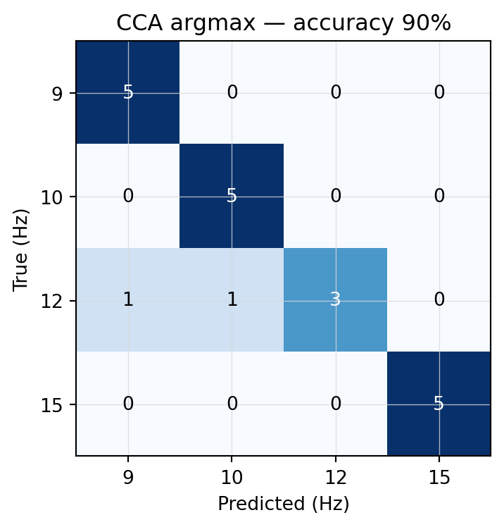
Figure 7.1: CCA-argmax confusion matrix. Cells show trial counts; cell shading is row-normalized (so the diagonal of a perfect classifier would be all-1.0).

The diagonal is mostly clean. The two errors are 12 Hz trials misread as 9 or 10 Hz — the same alpha-overlap pattern from Ch 2. FBCCA from Ch 6 picks up one of those (19/20 = 95 %), and we’ll include it in the head-to-head at the end of the chapter.

7.3 LDA on spectral SNR features

CCA scores are class-comparable by construction. The spectral SNR features from Ch 5 are not: a row’s “SNR at 9 Hz on Oz” sits in a different coordinate from “SNR at 10 Hz on Oz”, and there’s no a priori reason their absolute values are aligned across trials and classes. A trained classifier learns that mapping. Linear discriminant analysis (LDA) — the same family of model g.tec used to produce CH11 — is the natural baseline.

With only 20 trials and 64 features, we cross-validate leave-one-out: for each trial in turn, fit LDA on the other 19 and predict the held-out one.

def channel_psd(channel, fs, nperseg=NPERSEG):
    return welch(channel, fs=fs, nperseg=min(nperseg, len(channel)))


def snr_at(ff, pxx, f_target, half_bw_hz=0.6, neigh_hw_hz=2.5):
    df = ff[1] - ff[0]
    excl = max(1, int(round(half_bw_hz / df)))
    half = int(round(neigh_hw_hz / df))
    target = np.argmin(np.abs(ff - f_target))
    lo, hi = max(0, target - half), min(len(pxx), target + half + 1)
    idx = np.arange(lo, hi)
    idx = idx[np.abs(idx - target) > excl]
    return pxx[target] / pxx[idx].mean() if len(idx) else 0.0


def epoch_snr_features(epoch, fs):
    feats = []
    for ch in range(epoch.shape[0]):
        ff, pxx = channel_psd(epoch[ch], fs)
        for f in STIM_FREQS:
            for h in HARMONICS:
                feats.append(snr_at(ff, pxx, h * f))
    return np.array(feats)


X_snr = np.stack([epoch_snr_features(ep, fs) for ep in epochs])
print(f"X_snr: {X_snr.shape}  (n_trials, n_features)")

loo = LeaveOneOut()
lda_pred = np.zeros_like(labels)
for tr, te in loo.split(X_snr):
    lda = LinearDiscriminantAnalysis()
    lda.fit(X_snr[tr], labels[tr])
    lda_pred[te] = lda.predict(X_snr[te])

lda_acc = (lda_pred == labels).mean()
print(f"LDA on SNR features (LOO): {(lda_pred == labels).sum()}/{len(labels)} = {lda_acc:.0%}")

X_snr: (20, 64)  (n_trials, n_features)
LDA on SNR features (LOO): 11/20 = 55%

fig, ax = plt.subplots(figsize=(5, 4))
plot_confusion(confusion_matrix(labels, lda_pred, STIM_FREQS), STIM_FREQS,
               f"LDA on SNR — accuracy {lda_acc:.0%}", ax)
fig.tight_layout()
fig.savefig("images/07-classification_lda_confusion.png", dpi=200, bbox_inches="tight")
plt.show()

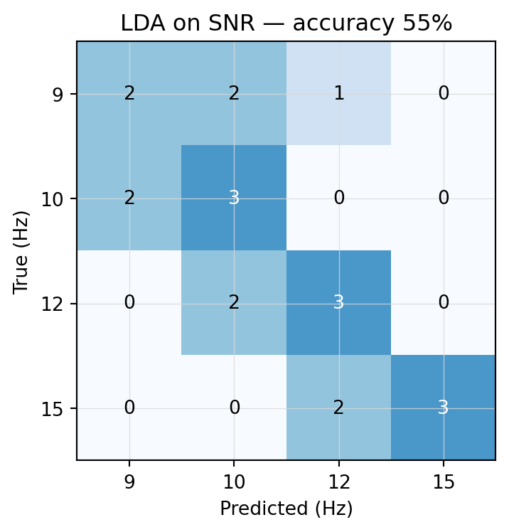
Figure 7.2: LDA on SNR features — leave-one-out predictions.

A long way short of CCA’s 90 %. With 64 features and only 19 training samples in each LOO fold, LDA is severely underdetermined — there are more features than samples, so the within-class covariance can’t be estimated reliably. The model is also blind to the phase information that CCA captures by construction. More features and more aggressive regularization could close some of the gap, but the core issue is that a generic classifier on top of a generic feature vector throws away the structure CCA exploits for free.

7.4 The CH11 baseline

CH11 is the LDA-class index that g.tec’s analysis tool wrote into the dataset at recording time — our shipped baseline. It fires intermittently (only when its confidence crosses a threshold), so per-trial prediction is the mode of the non-zero values within the trial window. The class indices map to frequencies via the parameters panel from Ch 1: 1 → 15 Hz, 2 → 12, 3 → 10, 4 → 9.

CH11_TO_HZ = {1: 15, 2: 12, 3: 10, 4: 9}


def ch11_predict(y, trials):
    ch11 = y[10].astype(int)
    preds = []
    for s, e, _ in trials:
        non_zero = ch11[s:e][ch11[s:e] != 0]
        if len(non_zero) == 0:
            preds.append(-1)  # no decision
        else:
            values, counts = np.unique(non_zero, return_counts=True)
            preds.append(CH11_TO_HZ.get(int(values[counts.argmax()]), -1))
    return np.array(preds)


ch11_pred = ch11_predict(y, trials)
ch11_acc = (ch11_pred == labels).mean()
print(f"CH11 (mode of non-zero samples): {(ch11_pred == labels).sum()}/{len(labels)} = {ch11_acc:.0%}")

CH11 (mode of non-zero samples): 11/20 = 55%

fig, ax = plt.subplots(figsize=(5, 4))
plot_confusion(confusion_matrix(labels, ch11_pred, STIM_FREQS), STIM_FREQS,
               f"CH11 — accuracy {ch11_acc:.0%}", ax)
fig.tight_layout()
fig.savefig("images/07-classification_ch11_confusion.png", dpi=200, bbox_inches="tight")
plt.show()

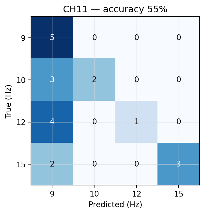
Figure 7.3: CH11 baseline — per-trial mode of non-zero samples.

CH11’s confusion matrix has a striking pattern: it falls back to 9 Hz for a lot of trials, regardless of the true class. The 9 Hz row is mostly correct (high recall for 9 Hz), but 10, 12, and 15 Hz rows leak heavily into the 9 Hz column (low precision elsewhere). Whatever the parameters g.tec used, the LDA on this session was strongly biased toward class 4. Worth noting: this is the same tool that produced a 100 %-stuck-on-class-3 baseline for subject_1_fvep_led_training_1 (Ch 1) — the g.tec analysis tool’s behaviour is brittle in ways that shipping it as a “result” obscures.

7.5 Three-way comparison

def fbcca_class_scores(epoch, fs, freqs=STIM_FREQS, sub_bands=SUB_BANDS,
                       a=1.25, b=0.25, n_harmonics=N_HARMONICS):
    n_samples = epoch.shape[1]
    weights = np.array([(i + 1) ** -a + b for i in range(len(sub_bands))])
    band_signals = []
    for low, high in sub_bands:
        b_, a_ = butter(4, [low, high], btype="band", fs=fs)
        band_signals.append(filtfilt(b_, a_, epoch, axis=-1))
    scores = np.zeros(len(freqs))
    for fi, freq in enumerate(freqs):
        Y = build_template(freq, n_samples, fs, n_harmonics)
        for bi, sig in enumerate(band_signals):
            scores[fi] += weights[bi] * cca_score(sig.T, Y) ** 2
    return scores


fbcca_pred = np.array([STIM_FREQS[fbcca_class_scores(ep, fs).argmax()] for ep in epochs])
fbcca_acc = (fbcca_pred == labels).mean()

methods = ["CH11", "LDA on SNR", "CCA argmax", "FBCCA argmax"]
accs = [ch11_acc, lda_acc, cca_acc, fbcca_acc]
print({m: f"{a:.0%}" for m, a in zip(methods, accs)})

{'CH11': '55%', 'LDA on SNR': '55%', 'CCA argmax': '90%', 'FBCCA argmax': '95%'}

colors = ["lightgray", "lightgray", "C2", "C2"]
fig, ax = plt.subplots(figsize=(8, 4))
bars = ax.bar(methods, accs, color=colors)
for bar, a in zip(bars, accs):
    ax.text(bar.get_x() + bar.get_width() / 2, a + 0.02, f"{a:.0%}",
            ha="center", fontsize=10)
ax.axhline(0.25, color="C3", ls="--", alpha=0.5, label="chance (25 %)")
ax.set_ylim(0, 1.05)
ax.set_ylabel("Accuracy")
ax.set_title("Classifier comparison — running session")
ax.legend(loc="upper left")
fig.tight_layout()
fig.savefig("images/07-classification_comparison.png", dpi=200, bbox_inches="tight")
plt.show()

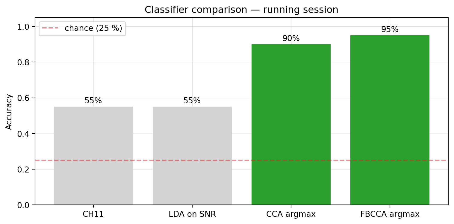
Figure 7.4: Per-trial accuracy across four classifiers on the running session (20 trials, chance = 25 %).

Two methods that match the structure of the SSVEP signal — CCA argmax and FBCCA argmax — clear 90 % with no training. Two methods that don’t — generic LDA on amplitude features, and the shipped CH11 LDA — sit roughly tied in the mid-50s, only modestly above chance. The lesson is the SSVEP literature’s main empirical finding: feature engineering that bakes in the physics of the response (narrowband, phase-locked, harmonic) lets a trivial classifier win. The “model” is the template; the argmax is a formality.

What we haven’t yet asked: how short can we make the epoch and still keep these accuracies? That’s Ch 8.