Apply the small amount of preprocessing SSVEP actually needs — a bandpass over the stimulation range and a notch at line frequency — and make a deliberate argument for why this is all we need. SSVEP is unusually robust compared to other EEG paradigms; this chapter explains why.
3.1 Back to the running example
Ch 2 borrowed subject_1_fvep_led_training_1.mat for visual intuition because the running file’s raw spectrum was dominated by the alpha rhythm and slow drift. With filtering in scope, the running example — subject_2_fvep_led_training_2.mat — returns from this chapter onward. Filtering doesn’t fix the alpha problem (more on that below), but it does take the drift out of the picture so the spectrum becomes readable.
3.2 What the unfiltered spectrum looks like
Code
from pathlib import Pathimport numpy as npimport scipy.ioimport matplotlib.pyplot as pltfrom scipy.signal import welch, butter, filtfilt, iirnotch, freqzDATA_DIR = Path("data")OZ =7mat = scipy.io.loadmat(DATA_DIR /"subject_2_fvep_led_training_2.mat")fs =int(mat["fs"][0, 0])y = mat["y"]oz_raw = y[OZ, fs:] # skip the first second (amplifier startup transient)ff_raw, pxx_raw = welch(oz_raw, fs=fs, nperseg=4096)print(f"Frequency resolution: {ff_raw[1] - ff_raw[0]:.3f} Hz")print(f"Power at 0.5 Hz: {pxx_raw[np.argmin(np.abs(ff_raw -0.5))]:.1f}")print(f"Power at 50 Hz : {pxx_raw[np.argmin(np.abs(ff_raw -50))]:.4f}")
Frequency resolution: 0.062 Hz
Power at 0.5 Hz: 134.9
Power at 50 Hz : 0.0012
Welch’s bin width is fs / nperseg — a longer segment buys finer frequency resolution at the cost of fewer segments to average, trading variance for sharpness. The window length chosen here keeps bins narrow enough that the four stimulation frequencies fall cleanly into distinct bins.
Code
fig, ax = plt.subplots(figsize=(11, 4.5))ax.semilogy(ff_raw, pxx_raw, lw=1)for f in [9, 10, 12, 15]: ax.axvline(f, color="C3", ls="--", alpha=0.3)ax.axvline(50, color="C1", ls="--", alpha=0.4, label="50 Hz (line)")ax.set_xlim(0, 80)ax.set_xlabel("Frequency (Hz)")ax.set_ylabel("Power (log)")ax.set_title("Oz, raw — full session")ax.legend()fig.tight_layout()fig.savefig("images/03-filtering_raw_psd.png", dpi=200, bbox_inches="tight")plt.show()
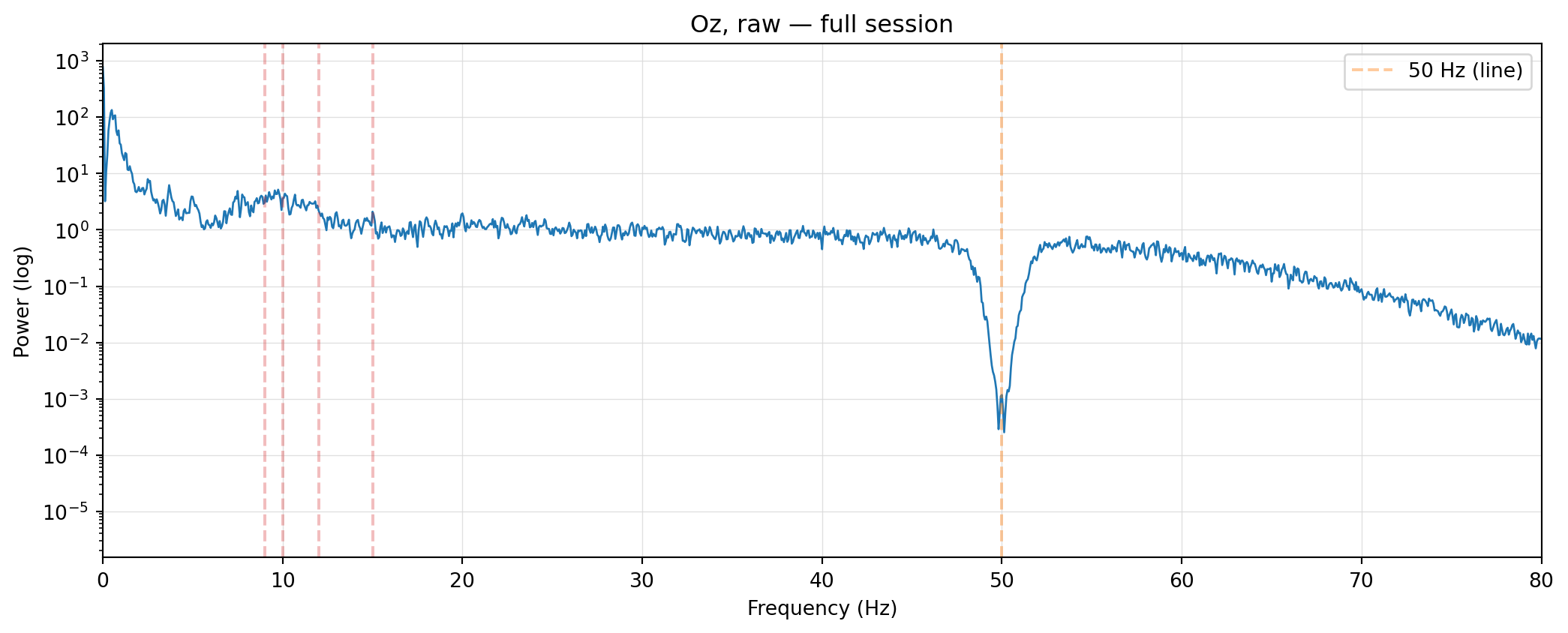
Figure 3.1: Long-window PSD on Oz, full session, log-y axis.
Two things stand out in the raw spectrum, neither of them the SSVEP. The biggest peak is at 0.5 Hz — slow baseline drift, amplified by the 1/f power law that EEG follows. Above ~40 Hz the spectrum drops off into the noise floor; the 50 Hz line-frequency spike that’s typically conspicuous in raw EEG isn’t there at all (power ≈ 0). The g.tec amplifier almost certainly applied its own front-end filtering before writing the file — convenient, but we’ll still design a notch for the same reason cars have seatbelts. The four stimulation frequencies (red dashes) sit inside the alpha band (8–13 Hz) and are barely distinguishable from the background.
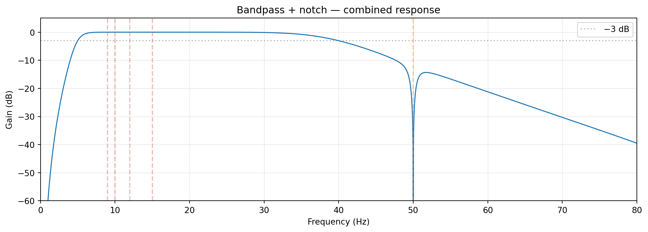
Figure 3.2: Combined bandpass (5–40 Hz, 4th-order Butterworth) and notch (50 Hz) frequency response.
Notice how clean this curve is compared to the raw PSD above — no jitter, no hairy line. That’s because this isn’t an estimate from data; freqz evaluates the filter’s transfer function analytically from its coefficients, so there’s no variance to average down. It’s what the filter does by construction, not what we measured.
The passband at 5–40 Hz comfortably covers the four fundamentals (9, 10, 12, 15 Hz) and the second harmonics of the lower three (18, 20, 24 Hz) — the harmonic of 15 Hz at 30 Hz also gets through. We use filtfilt for zero phase (forward + reverse pass) so the SSVEP’s phase relative to the stimulus isn’t smeared, and a 4th-order Butterworth so the passband is flat (no ripple riding on top of the SSVEP peaks). The 50 Hz notch is narrow (Q = 30) — defensive even though there’s nothing there to remove on this file.
3.4 Before and after — spectrum
Code
ff_filt, pxx_filt = welch(oz_filt, fs=fs, nperseg=4096)fig, ax = plt.subplots(figsize=(11, 4.5))ax.semilogy(ff_raw, pxx_raw, lw=1, alpha=0.5, label="raw")ax.semilogy(ff_filt, pxx_filt, lw=1, label="filtered")for f in [9, 10, 12, 15]: ax.axvline(f, color="C3", ls="--", alpha=0.3)ax.set_xlim(0, 80)ax.set_xlabel("Frequency (Hz)")ax.set_ylabel("Power (log)")ax.set_title("Oz — raw vs filtered")ax.legend()fig.tight_layout()fig.savefig("images/03-filtering_bef_aft_psd.png", dpi=200, bbox_inches="tight")plt.show()
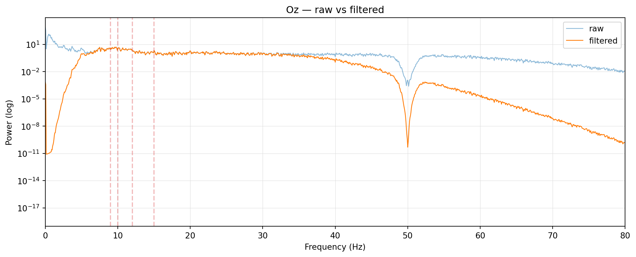
Figure 3.3: Oz PSD, raw vs filtered, full session, log-y.
The drift below ~3 Hz drops by orders of magnitude; everything above ~45 Hz drops into numerical noise; in between the two spectra are the same. This is what filtering does — and only what filtering does. Inside the passband the per-sample values are unchanged by Butterworth filtering (its passband is flat by construction), so the alpha rhythm at ~10 Hz is still right where it was, the SSVEP peaks are still where they were, and the SNR between them is identical. Filtering makes the spectrum readable; it doesn’t change what’s in the analysis band.
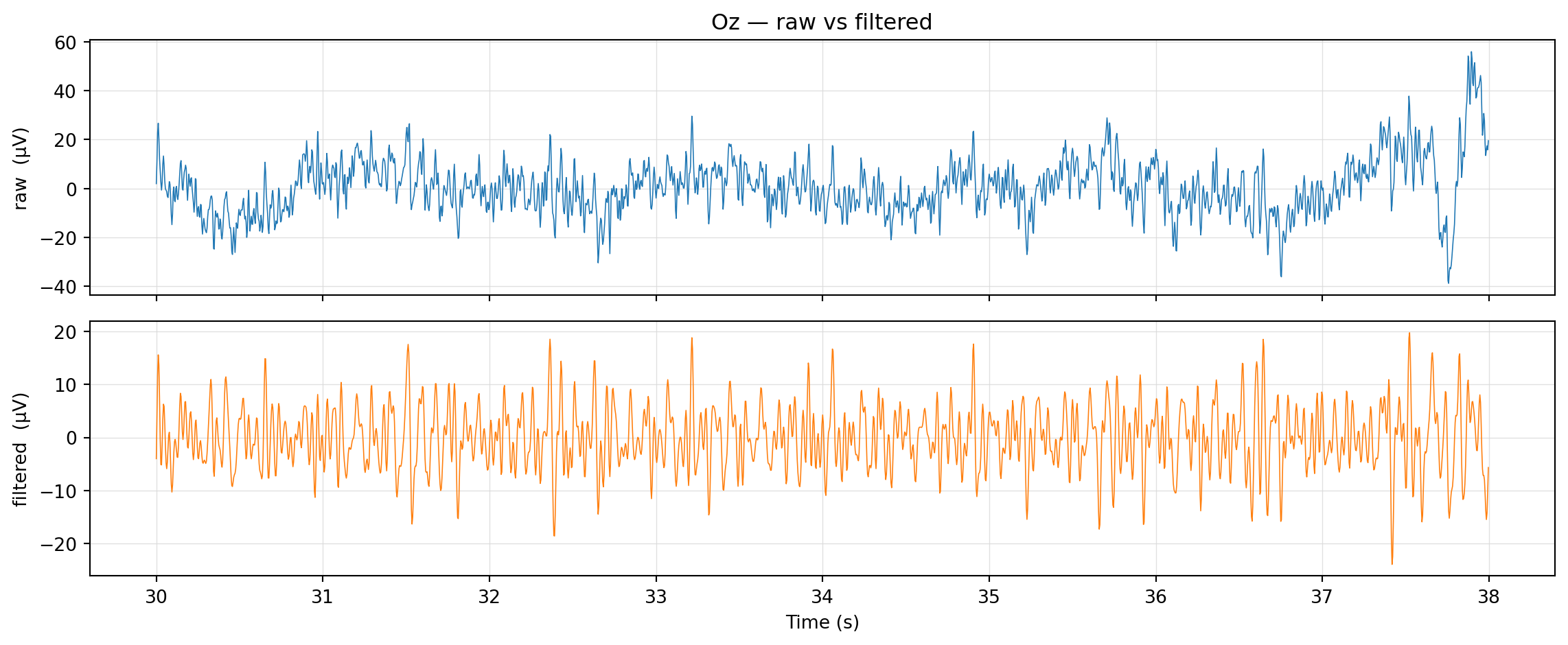
Figure 3.4: Same 8-second window of Oz, raw vs filtered.
The raw trace wanders around a slowly-shifting baseline — the few slow cycles you can count across the window are consistent with the sub-1 Hz drift the PSD flagged — while the filtered trace sits cleanly around zero. The fast oscillations — the part that actually carries the SSVEP — look effectively identical. Removing the drift matters most for time-domain features (per-trial means and amplitudes) and for any feature that’s sensitive to absolute level; for spectral features it’s almost cosmetic.
3.6 Why this is enough — and what it doesn’t fix
Compared to motor-imagery or P300 paradigms, SSVEP needs almost no preprocessing. The response is generated in a small, well-localized region of cortex (V1/V2), it’s narrowband and phase-locked to the stimulus, and the band it lives in (~9–30 Hz including harmonics) doesn’t overlap with the worst contaminants — eye blinks live below 4 Hz and muscle activity above 40 Hz, both safely outside the passband. Heavy artifact removal (ICA, regression-based EOG correction, full re-referencing pipelines) is overkill here and risks subtracting out signal you wanted to keep.
What filtering on this file doesn’t fix is the alpha rhythm sitting on top of the lower stimulation frequencies (9, 10, 12 Hz) — that’s a within-passband collision and no linear filter will untangle it. Two later chapters handle it differently. Ch 5 builds SNR features that normalize each peak by its neighbourhood, so an alpha bump that’s tall but flanked by similarly tall bins gets deflated relative to a peak that genuinely stands out. Ch 6 takes a phase-aware route: CCA against sine/cosine references at the stimulation frequencies. The SSVEP is phase-locked to the LED, alpha isn’t, so the correlation with a 10 Hz template behaves very differently for an actual 10 Hz stimulation trial than it does for spontaneous 10 Hz alpha — even though both have a peak at 10 Hz in the PSD.
3.7 Frequency vs phase — a small demo
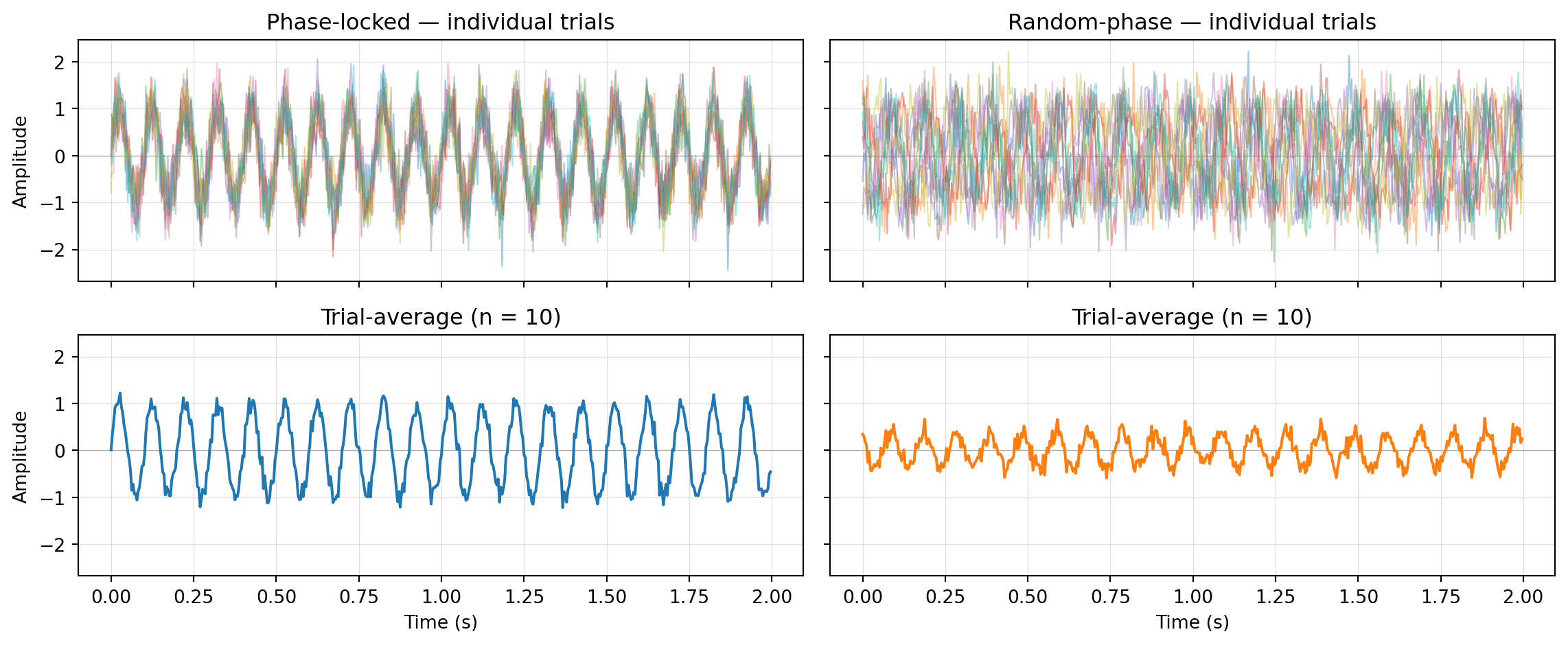
To make the phase point concrete, here’s a small synthetic demo: two sets of trials, every trial a 10 Hz sinusoid in noise. In one set every trial starts at the same phase — the SSVEP analogue, locked to a stimulus. In the other, each trial’s starting phase is drawn uniformly at random — the alpha analogue, spontaneous and unanchored.
Figure 3.5: Two sets of synthetic 10 Hz trials in noise. Top: individual trials overlaid. Bottom: the trial-average. The phase-locked mean preserves the oscillation; the random-phase mean collapses toward zero.
Individually, every trial in either column is a 10 Hz oscillation in noise — a per-trial PSD would put a peak at 10 Hz for both, and a frequency-only feature would call them indistinguishable. The difference only emerges once trials are combined: phase-locked trials reinforce each other and the average preserves the oscillation, while random-phase trials interfere destructively and the average collapses toward zero. The PSD discards exactly the information — phase — that separates the two. Methods that keep it (trial-averaging, template correlation, coherence with a stimulus reference) have something extra to work with; methods that don’t, don’t. Ch 6 develops this into a working classifier.
To check whether the same effect actually shows up on the running session, swap the synthetic trials for the real ones. Bandpass Oz tightly around 10 Hz to isolate the alpha/SSVEP-at-10-Hz band, then for each of the five 10 Hz trials take two paired segments of equal length: the trial itself starting at the CH10 trigger edge (the SSVEP candidate) and the rest window immediately before that trigger (the alpha candidate, since the LED is still off and there’s no shared zero-time tying alpha to anything). Same n on both sides keeps the averaging comparison fair.
Code
bp_alpha = butter(4, [8, 12], btype="band", fs=fs)oz_alpha = filtfilt(*bp_alpha, y[OZ].astype(float))ch10 = y[9].astype(int)edges = np.diff((ch10 !=0).astype(int))trial_starts = np.where(edges ==1)[0] +1trial_ends = np.where(edges ==-1)[0] +1inter_trial_gaps = trial_starts[1:] - trial_ends[:-1]SEG_LEN =int(inter_trial_gaps.min()) # rest-gap length, set by the g.tec scheduleten_hz_starts = [s for s in trial_starts if ch10[s] ==10]ssvep_real = np.array([oz_alpha[s:s + SEG_LEN] for s in ten_hz_starts])alpha_real = np.array([oz_alpha[s - SEG_LEN:s] for s in ten_hz_starts if s >= SEG_LEN])print(f"Segment length: {SEG_LEN / fs:.2f} s")print(f"ssvep_real: {ssvep_real.shape}, alpha_real: {alpha_real.shape}")
Segment length: 3.14 s
ssvep_real: (5, 805), alpha_real: (5, 805)
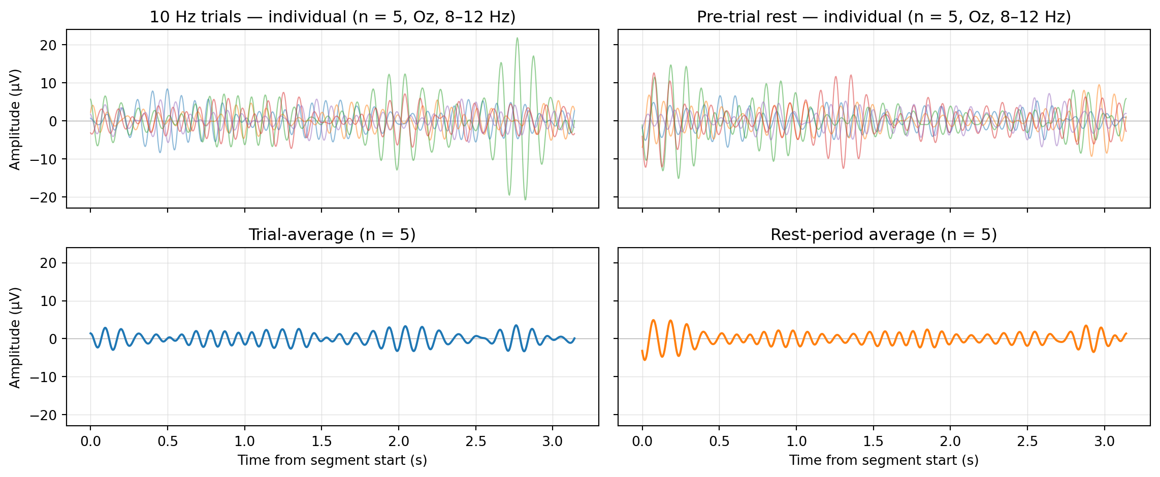
Figure 3.6: Same demo on the running session: Oz bandpassed at 8–12 Hz. Left: 10 Hz stimulation trials aligned to CH10 trigger onset. Right: inter-trial rest segments aligned to end-of-previous-trial. Top row: individual segments overlaid. Bottom row: their averages.
How clean the contrast looks depends on the session. The trial-average should preserve a visible 10 Hz oscillation across cycles; the rest-average — same n, same length, just no trigger-anchored signal underneath — should sit closer to zero, with no consistent phase to lock onto. If the rest-average still wobbles, that’s expected at n = 5: alpha doesn’t cancel hard with so few segments, and on this subject the alpha rhythm is weaker than on the alpha-dominated subject 1 used in Ch 2 — so there’s less amplitude for destructive interference to cancel in the first place. Whatever the visible margin, it’s the dataset’s own version of the synthetic demo above. Ch 6 develops this into a working classifier.