5  Spectral Features

Turn each epoch into a feature vector a classifier can use. The most direct route for SSVEP: compute a PSD per epoch, sample the amplitude at each candidate stimulation frequency and its harmonics, and stack those into a feature row.

5.1 Setup: load, filter, epoch

The pipeline from Ch 3 + Ch 4 in compact form: load the running session, bandpass + notch the eight EEG channels, build the (n_trials, 8, n_samples) epoch tensor.

from pathlib import Path
import numpy as np
import scipy.io
import matplotlib.pyplot as plt
from matplotlib.colors import LogNorm
from scipy.signal import welch, butter, filtfilt, iirnotch
import mne
mne.set_log_level("WARNING")

DATA_DIR = Path("data")
EEG_LABELS = ["PO7", "PO3", "POz", "PO4", "PO8", "O1", "Oz", "O2"]
STIM_FREQS = [9, 10, 12, 15]
HARMONICS = [1, 2]

mat = scipy.io.loadmat(DATA_DIR / "subject_2_fvep_led_training_2.mat")
fs = int(mat["fs"][0, 0])
y = mat["y"]


def make_filters(fs, low=5.0, high=40.0, line=50.0, order=4, notch_q=30):
    bp_b, bp_a = butter(order, [low, high], btype="band", fs=fs)
    n_b, n_a = iirnotch(line, notch_q, fs=fs)
    return (bp_b, bp_a), (n_b, n_a)


def apply_filters(x, bp, notch):
    return filtfilt(*notch, filtfilt(*bp, x))


def find_trials(y):
    ch10 = y[9].astype(int)
    active = (ch10 != 0).astype(int)
    diff = np.diff(active)
    starts = np.where(diff == 1)[0] + 1
    ends = np.where(diff == -1)[0] + 1
    return [(int(s), int(e), int(ch10[s])) for s, e in zip(starts, ends)]


bp, notch = make_filters(fs)
y_filt = y.astype(float).copy()
for ci in range(1, 9):
    y_filt[ci] = apply_filters(y[ci], bp, notch)

trials = find_trials(y)
n_samples = trials[0][1] - trials[0][0]
epochs = np.stack([y_filt[1:9, s:s + n_samples] for s, _, _ in trials])
labels = np.array([fr for _, _, fr in trials])
print(f"epochs: {epochs.shape}, labels: {labels.shape}")

epochs: (20, 8, 1883), labels: (20,)

5.2 From an epoch to a feature vector

For each of the eight EEG channels we compute Welch’s PSD on the epoch, then read off the amplitude at each candidate stimulation frequency (9, 10, 12, 15 Hz) and its second harmonic (18, 20, 24, 30 Hz). That’s eight values per channel × eight channels = 64 features per trial.

NPERSEG = 512  # 0.5 Hz resolution at fs = 256 Hz


def channel_psd(channel, fs, nperseg=NPERSEG):
    return welch(channel, fs=fs, nperseg=min(nperseg, len(channel)))


def epoch_features(epoch, fs):
    """Return a (n_channels * len(STIM_FREQS) * len(HARMONICS),) feature vector."""
    feats = []
    for ch in range(epoch.shape[0]):
        ff, pxx = channel_psd(epoch[ch], fs)
        for f in STIM_FREQS:
            for h in HARMONICS:
                feats.append(pxx[np.argmin(np.abs(ff - h * f))])
    return np.array(feats)


print(f"Feature vector for epochs[0]: shape = {epoch_features(epochs[0], fs).shape}")

Feature vector for epochs[0]: shape = (64,)

ep_idx = 0
ep = epochs[ep_idx]
ep_label = labels[ep_idx]

# (channel index, freq to mark, label, text offset in points)
HIGHLIGHTS = [
    (6, 15, "clean f", (14, 6)),       # Oz — fundamental
    (7, 30, "2f dominates", (-78, 0)), # O2 — harmonic flip
]

fig, axes = plt.subplots(2, 4, figsize=(14, 6), sharey=True)
for ci, ax in enumerate(axes.ravel()):
    ff, pxx = channel_psd(ep[ci], fs)
    ax.plot(ff, pxx, lw=0.9)
    for f in STIM_FREQS:
        ax.axvline(f, color="C3", ls="--", alpha=0.6, lw=0.9)
        ax.axvline(2 * f, color="C2", ls=":", alpha=0.9, lw=1.1)
    for h_ci, h_f, h_label, h_off in HIGHLIGHTS:
        if h_ci == ci:
            bin_i = np.argmin(np.abs(ff - h_f))
            ax.annotate(
                h_label, xy=(ff[bin_i], pxx[bin_i]),
                xytext=h_off, textcoords="offset points",
                fontsize=8, color="0.2",
                arrowprops=dict(arrowstyle="->", lw=0.8, color="0.2"),
            )
    ax.set_xlim(5, 35)
    ax.set_title(EEG_LABELS[ci], fontsize=9)
    ax.tick_params(labelsize=7)
for ax in axes[-1]:
    ax.set_xlabel("Frequency (Hz)")
for ax in axes[:, 0]:
    ax.set_ylabel("Power")
fig.suptitle(f"Trial {ep_idx} — {ep_label} Hz stim", fontsize=10)
fig.tight_layout()
fig.savefig("images/05-spectral-features_one_trial.png", dpi=200, bbox_inches="tight")
plt.show()

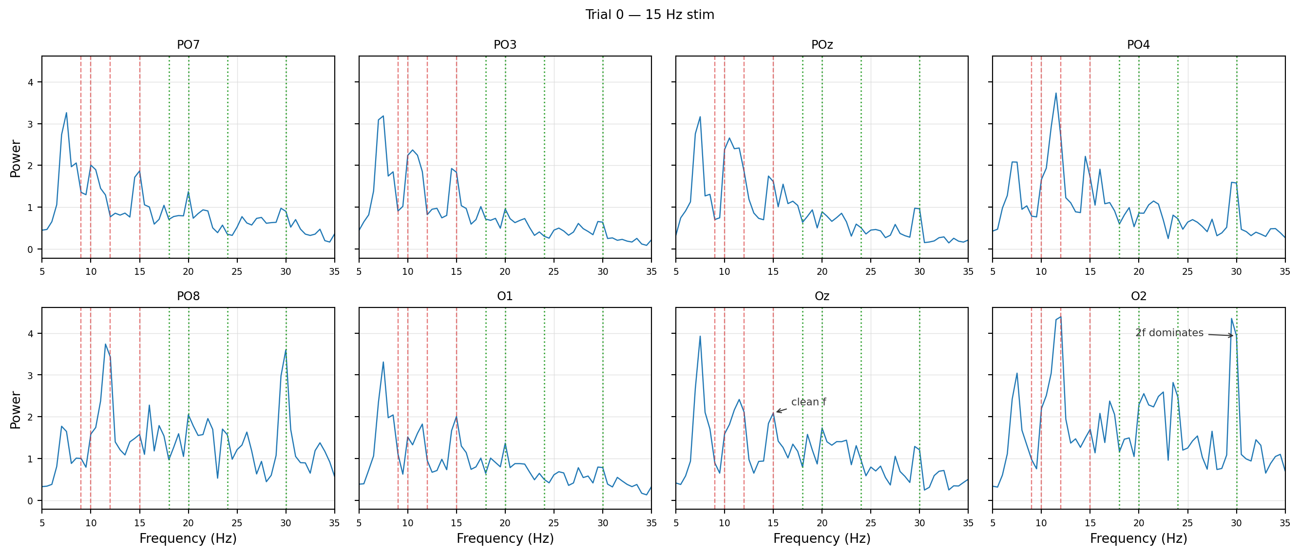
Figure 5.1: Per-channel PSD for one epoch (15 Hz class). Red dashed lines mark the four fundamentals; green dotted lines mark the four second harmonics. The classifier sees the PSD value at each of these eight frequencies on each of the eight channels.

For this 15 Hz trial the cleanest peaks at 15 Hz are on Oz, O1, PO7 and PO3 — occipital and left-lateralized. The right-side channels (O2, PO8) have a fat neighbourhood around 15 Hz that almost swallows the peak. Strikingly, the 30 Hz harmonic flips the picture: it’s small on the left channels but dominant on the right (on O2 and PO8 the 30 Hz peak is more than twice the 15 Hz fundamental). So the fundamental and the harmonic carry different spatial information on the same trial — another reason to keep all eight channels and both harmonics in the feature vector rather than betting everything on Oz at f.

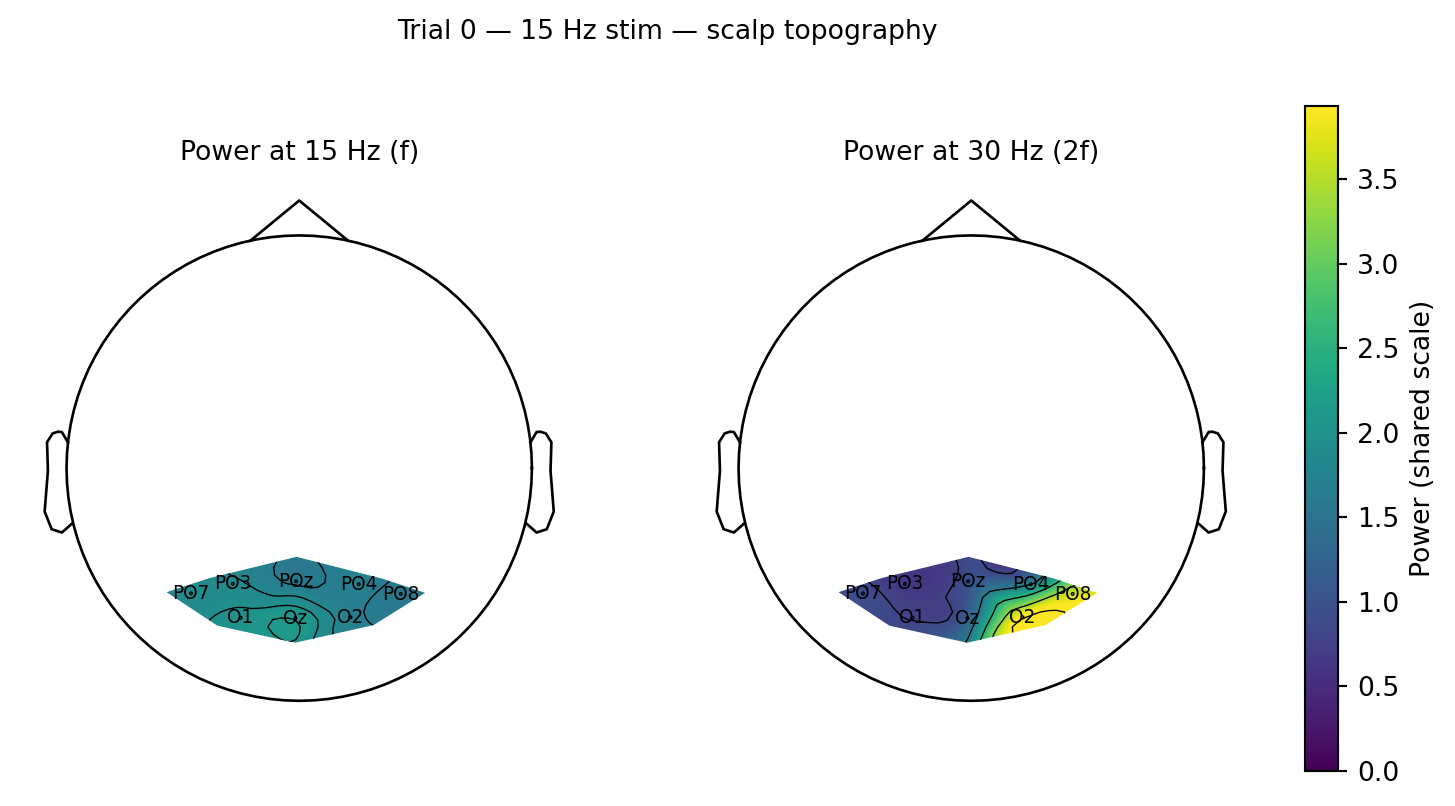
The same eight numbers, viewed on the scalp, make this even more vivid:

ff_ch, pxx_ch = welch(ep, fs=fs, nperseg=min(NPERSEG, ep.shape[1]))
p15 = pxx_ch[:, np.argmin(np.abs(ff_ch - 15))]
p30 = pxx_ch[:, np.argmin(np.abs(ff_ch - 30))]

info = mne.create_info(ch_names=EEG_LABELS, sfreq=fs, ch_types="eeg")
info.set_montage(mne.channels.make_standard_montage("standard_1020"))

vmax = max(p15.max(), p30.max())
fig, axes = plt.subplots(1, 2, figsize=(9, 4.5))
for ax, vals, title in [(axes[0], p15, "Power at 15 Hz (f)"),
                         (axes[1], p30, "Power at 30 Hz (2f)")]:
    im, _ = mne.viz.plot_topomap(vals, info, axes=ax, show=False,
                                  names=EEG_LABELS, cmap="viridis",
                                  contours=4, sensors=True,
                                  extrapolate="local",
                                  vlim=(0, vmax))
    ax.set_title(title, fontsize=10)
fig.colorbar(im, ax=axes, fraction=0.04, pad=0.04, label="Power (shared scale)")
fig.suptitle(f"Trial {ep_idx} — {ep_label} Hz stim — scalp topography", fontsize=10)
fig.savefig("images/05-spectral-features_topomap.png", dpi=200, bbox_inches="tight")
plt.show()

Figure 5.2: Scalp topography of band power for the same epoch, restricted to the convex hull of the eight electrodes and on a shared colour scale so the two bands are directly comparable. Left: the 15 Hz fundamental sits broadly across occipital cortex with a left bias. Right: the 30 Hz harmonic is sharply lateralized to the right (O2/PO8) and outside that hot spot is weaker than the fundamental.

A static topography averages over the whole 7.5 s epoch and hides any time evolution. Sliding a short window through the trial and re-rendering both topomaps frame-by-frame shows where and when the response actually builds up.

Figure 5.3: Sliding 1.5 s window (0.5 s hop) through the 7.5 s trial. Both panels share a colour scale derived from the per-window maximum across both bands, so brightness is directly comparable across frames and bands. The 15 Hz response appears almost immediately and stays broadly distributed; the 30 Hz response builds up later and concentrates on the right occipital electrodes.

Sampling at expected frequencies — rather than feeding the entire 5–40 Hz spectrum to the classifier — collapses each PSD to a small, physically meaningful number of values: it bakes in what we know about the experiment, gives the model fewer features to overfit to, and is robust to per-trial scaling differences.

5.3 The feature matrix for a whole session

feat_matrix = np.stack([epoch_features(epochs[i], fs) for i in range(len(epochs))])
print(f"feat_matrix shape: {feat_matrix.shape}  (n_trials, n_channels × n_stimulation_frequencies × n_harmonics)")

feat_matrix shape: (20, 64)  (n_trials, n_channels × n_stimulation_frequencies × n_harmonics)

order = np.lexsort((np.arange(len(labels)), labels))
sorted_feat = feat_matrix[order]
sorted_labels = labels[order]

n_per_block = 8  # 8 channels sampled at each (stimulation frequency, harmonic)
group_labels = [f"{h * f} Hz" for f in STIM_FREQS for h in HARMONICS]

fig, ax = plt.subplots(figsize=(13, 5))
im = ax.imshow(sorted_feat, aspect="auto", origin="upper",
               cmap="viridis", norm=LogNorm())
for i in range(1, len(group_labels)):
    ax.axvline(i * n_per_block - 0.5, color="white", lw=0.8)
class_changes = np.where(np.diff(sorted_labels) != 0)[0] + 0.5
for r in class_changes:
    ax.axhline(r, color="white", lw=0.8)
ax.set_xticks([i * n_per_block + n_per_block / 2 - 0.5 for i in range(len(group_labels))])
ax.set_xticklabels(group_labels)
ax.set_xlabel("Feature group  (eight channels sampled at each frequency)")
yt = [np.where(sorted_labels == c)[0].mean() for c in sorted(set(sorted_labels))]
ax.set_yticks(yt)
ax.set_yticklabels([f"{c} Hz" for c in sorted(set(sorted_labels))])
ax.set_ylabel("Trial class (5 trials each)")
fig.colorbar(im, ax=ax, label="Power (log scale)")
fig.tight_layout()
fig.savefig("images/05-spectral-features_matrix.png", dpi=200, bbox_inches="tight")
plt.show()

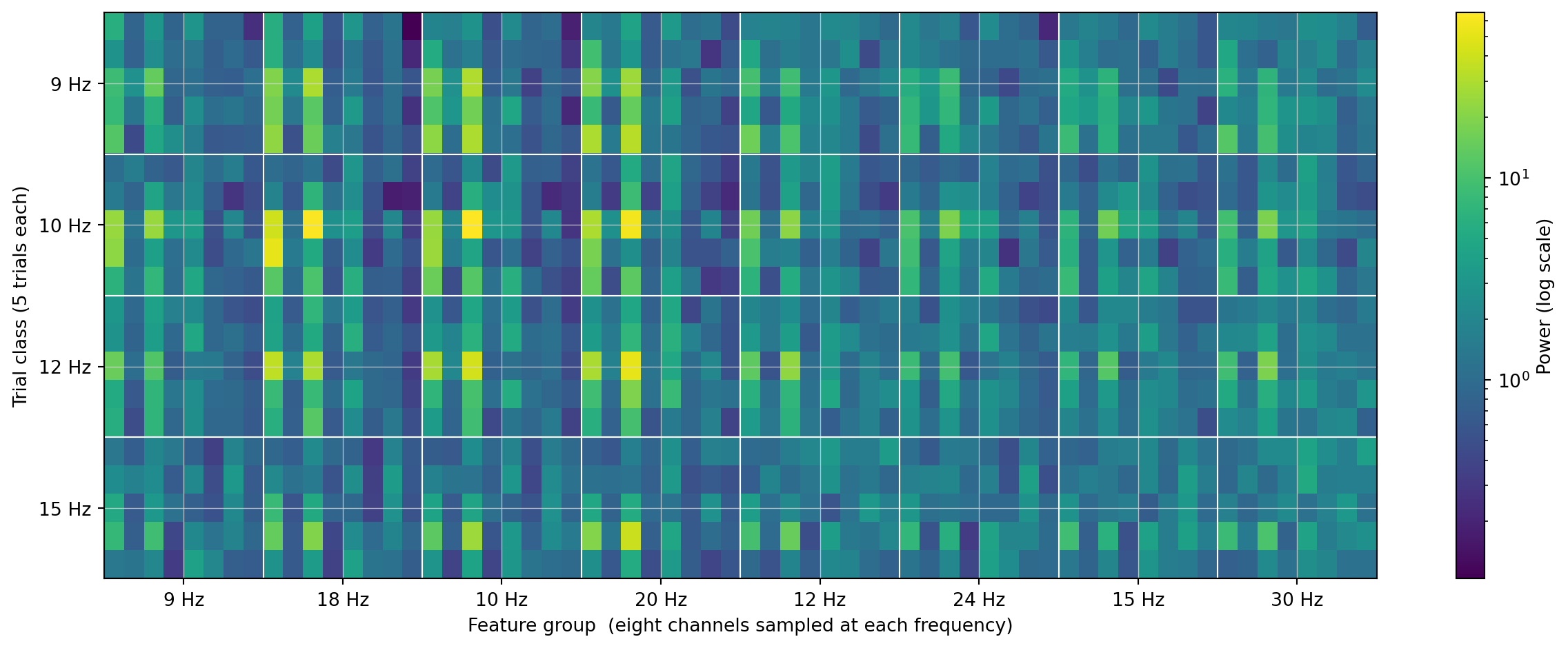
Figure 5.4: Feature matrix, rows sorted by stimulation class. Each row is one trial; each column is one (channel, frequency, harmonic) feature. Vertical lines separate frequency-and-harmonic groups.

How to read this heatmap: each row is one trial, each column is one of the 64 features (8 channels × 8 sampled frequencies). Rows are sorted so the five 9 Hz trials sit at the top, then the 10, 12, and 15 Hz blocks below. Columns are grouped by sampled frequency — the leftmost eight columns are all “PSD power at 9 Hz, one per channel”; the next eight are “PSD power at 18 Hz” (the second harmonic of 9 Hz); and so on through 30 Hz.

Class structure shows up as bright cells lining up along the column whose frequency matches the row’s class. The top five rows (9 Hz) are brightest in the 9 Hz column block — exactly where you’d expect — and you can also see them light up in the 18 Hz column block, which is the second harmonic. That’s the harmonics earning their place in the feature vector: they fire independently of the fundamental, adding evidence rather than duplicating it. The 10 Hz row block follows the same pattern at 10 and 20 Hz. Where the eye can already separate the classes from the matrix alone, a linear classifier almost certainly can too.

The 12 and 15 Hz row blocks look noticeably dimmer than 9 and 10 Hz — same story as Ch 2: those classes have weaker raw-power features on this subject (12 Hz overlaps with alpha, 15 Hz drives a smaller harmonic). The classifier has less to work with there.

5.4 A strawman classifier

Before reaching for fancier features, ask the simplest possible question: how far does raw power on its own get you? For each trial, sum the feature row over channels and harmonics per stimulation frequency, then pick the frequency with the most total power. No training, no normalization, no model — pure argmax over the matrix above.

power_per_freq = feat_matrix.reshape(
    len(epochs), len(EEG_LABELS), len(STIM_FREQS), len(HARMONICS)
).sum(axis=(1, 3))
naive_pred = np.array([STIM_FREQS[i] for i in power_per_freq.argmax(axis=1)])
naive_acc = (naive_pred == labels).mean()
print(f"Raw-power argmax: {(naive_pred == labels).sum()}/{len(labels)} = {naive_acc:.0%}")

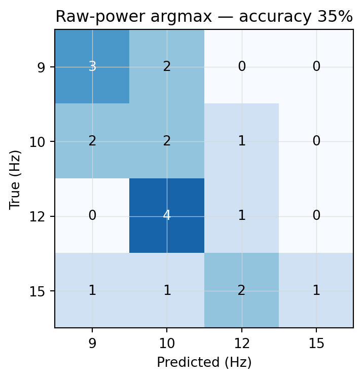
Raw-power argmax: 7/20 = 35%

cm = np.zeros((len(STIM_FREQS), len(STIM_FREQS)), dtype=int)
for t, p in zip(labels, naive_pred):
    cm[STIM_FREQS.index(int(t)), STIM_FREQS.index(int(p))] += 1
cm_norm = cm / np.maximum(cm.sum(axis=1, keepdims=True), 1)

fig, ax = plt.subplots(figsize=(5, 4))
ax.imshow(cm_norm, cmap="Blues", vmin=0, vmax=1)
for i in range(len(STIM_FREQS)):
    for j in range(len(STIM_FREQS)):
        ax.text(j, i, f"{cm[i, j]}", ha="center", va="center", fontsize=10,
                color="white" if cm_norm[i, j] > 0.5 else "black")
ax.set_xticks(range(len(STIM_FREQS)))
ax.set_xticklabels([str(f) for f in STIM_FREQS])
ax.set_yticks(range(len(STIM_FREQS)))
ax.set_yticklabels([str(f) for f in STIM_FREQS])
ax.set_xlabel("Predicted (Hz)")
ax.set_ylabel("True (Hz)")
ax.set_title(f"Raw-power argmax — accuracy {naive_acc:.0%}")
fig.tight_layout()
fig.savefig("images/05-spectral-features_naive_confusion.png", dpi=200, bbox_inches="tight")
plt.show()

Figure 5.5: Raw-power argmax — confusion matrix. Cells show trial counts; shading is row-normalized.

The diagonal is uneven. Classes whose fundamental sits inside the alpha band bleed into each other in the predictable way: raw power can’t tell a true 10 Hz SSVEP peak apart from spontaneous 10 Hz alpha — both are just a bin with high power. Something needs to weigh peaks against their local background, not just measure their absolute height.

5.5 SNR features

Raw amplitude features are sensitive to the per-trial overall level — attention, electrode drift across the session, residual 1/f tilt. We can normalize each sampled bin by the average amplitude in its neighbourhood, turning power into a signal-to-noise ratio. The peak still has to stand out against its background, not merely be tall in absolute terms.

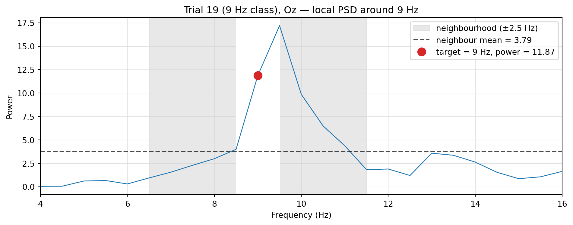
To make the transformation concrete, take a single cell from the matrix above: the 9 Hz feature on Oz for the last 9 Hz trial (one of the cleanest single-trial SSVEPs in the session). Here’s its local PSD around 9 Hz:

ti, ch_idx, f_target = 19, 7, 9.0
ff_ex, pxx_ex = channel_psd(epochs[ti, ch_idx], fs)
df = ff_ex[1] - ff_ex[0]
target_bin = np.argmin(np.abs(ff_ex - f_target))
half_bw_hz, neigh_hw_hz = 0.6, 2.5
excl_bins = max(1, int(round(half_bw_hz / df)))
half_bins = int(round(neigh_hw_hz / df))
lo = max(0, target_bin - half_bins)
hi = min(len(pxx_ex), target_bin + half_bins + 1)
neigh_idx = np.arange(lo, hi)
neigh_idx = neigh_idx[np.abs(neigh_idx - target_bin) > excl_bins]

target_p = pxx_ex[target_bin]
neigh_mean = pxx_ex[neigh_idx].mean()

fig, ax = plt.subplots(figsize=(10, 4))
ax.plot(ff_ex, pxx_ex, lw=1.0)
ax.axvspan(ff_ex[lo], ff_ex[min(hi - 1, len(ff_ex) - 1)], color="lightgray",
           alpha=0.5, label="neighbourhood (±2.5 Hz)")
ax.axvspan(ff_ex[max(0, target_bin - excl_bins)], ff_ex[min(len(ff_ex) - 1, target_bin + excl_bins)],
           color="white", alpha=1.0)
ax.axhline(neigh_mean, color="k", ls="--", alpha=0.7,
           label=f"neighbour mean = {neigh_mean:.2f}")
ax.plot(ff_ex[target_bin], target_p, "o", color="C3", ms=10,
        label=f"target = {f_target:.0f} Hz, power = {target_p:.2f}")
ax.set_xlim(4, 16)
ax.set_xlabel("Frequency (Hz)")
ax.set_ylabel("Power")
ax.set_title(f"Trial {ti} ({labels[ti]} Hz class), Oz — local PSD around {f_target:.0f} Hz")
ax.legend(loc="upper right")
fig.tight_layout()
fig.savefig("images/05-spectral-features_snr_example.png", dpi=200, bbox_inches="tight")
plt.show()

print(f"  raw power:           {target_p:.2f}")
print(f"  neighbour mean:      {neigh_mean:.2f}")
print(f"  SNR  =  {target_p:.2f} / {neigh_mean:.2f}  =  {target_p / neigh_mean:.2f}")

Figure 5.6: Local PSD on Oz for the last 9 Hz trial. The target bin (red) sits well above the average of its flanking neighbours (dashed line) — the SNR feature is the ratio of the two.

  raw power:           11.87
  neighbour mean:      3.79
  SNR  =  11.87 / 3.79  =  3.13

The target sits about 3× above its background — that’s the SNR feature value for this single cell. The same calculation runs across all 64 (channel × frequency) entries of the matrix.

Note

Why ±2.5 Hz for the neighbourhood? A balance between two pressures. Wide enough to span the alpha bump (itself ~2–3 Hz wide) so alpha doesn’t get counted as “signal” sitting right next to its target, and to leave enough bins for a stable noise mean. Narrow enough that EEG’s 1/f tilt doesn’t average across very different noise regimes (the floor at 9 Hz is genuinely higher than at 30 Hz), and to keep the band clear of neighbouring harmonic families — for f = 15 Hz, the 12.5–17.5 Hz neighbourhood stops short of 18 Hz, which is the 2f harmonic of the 9 Hz class. The ±0.6 Hz exclusion carves out the target peak itself plus its Welch-leakage skirts. Adjacent stim classes are as close as 1 Hz apart, so other stim frequencies do fall inside the band — that’s fine because only one class is driven per trial, so there’s no rival peak to pollute the estimate.

What does the transformation actually do? Take a contrasting cell from the same trial: the 12 Hz feature on Oz has raw power 1.89 (small) but its neighbourhood includes the alpha bump near 10 Hz, so the neighbour mean is 6.13. Their ratio is 0.31 — well below 1, signalling “this bin sits below its surroundings”, i.e. there is no SSVEP peak at 12 Hz on this trial. Raw power can’t make that distinction; SNR can. The cell’s pre/post values: raw = 1.89, SNR = 0.31. Both numbers go into the heatmap as “low”, but the SNR version is more committed about it.

def snr_at(ff, pxx, f_target, half_bw_hz=0.6, neigh_hw_hz=2.5):
    """Power at the target bin / mean power in a flanking neighborhood,
    excluding ±half_bw_hz around the target."""
    df = ff[1] - ff[0]
    excl = max(1, int(round(half_bw_hz / df)))
    half = int(round(neigh_hw_hz / df))
    target = np.argmin(np.abs(ff - f_target))
    lo, hi = max(0, target - half), min(len(pxx), target + half + 1)
    idx = np.arange(lo, hi)
    idx = idx[np.abs(idx - target) > excl]
    if len(idx) == 0:
        return 0.0
    return pxx[target] / pxx[idx].mean()


def epoch_snr_features(epoch, fs):
    feats = []
    for ch in range(epoch.shape[0]):
        ff, pxx = channel_psd(epoch[ch], fs)
        for f in STIM_FREQS:
            for h in HARMONICS:
                feats.append(snr_at(ff, pxx, h * f))
    return np.array(feats)


snr_matrix = np.stack([epoch_snr_features(epochs[i], fs) for i in range(len(epochs))])
print(f"snr_matrix shape: {snr_matrix.shape}")

snr_matrix shape: (20, 64)

sorted_snr = snr_matrix[order]

fig, ax = plt.subplots(figsize=(13, 5))
im = ax.imshow(sorted_snr, aspect="auto", origin="upper", cmap="viridis")
for i in range(1, len(group_labels)):
    ax.axvline(i * n_per_block - 0.5, color="white", lw=0.8)
for r in class_changes:
    ax.axhline(r, color="white", lw=0.8)
ax.set_xticks([i * n_per_block + n_per_block / 2 - 0.5 for i in range(len(group_labels))])
ax.set_xticklabels(group_labels)
ax.set_xlabel("Feature group  (eight channels sampled at each frequency)")
ax.set_yticks(yt)
ax.set_yticklabels([f"{c} Hz" for c in sorted(set(sorted_labels))])
ax.set_ylabel("Trial class (5 trials each)")
fig.colorbar(im, ax=ax, label="SNR")
fig.tight_layout()
fig.savefig("images/05-spectral-features_snr_matrix.png", dpi=200, bbox_inches="tight")
plt.show()

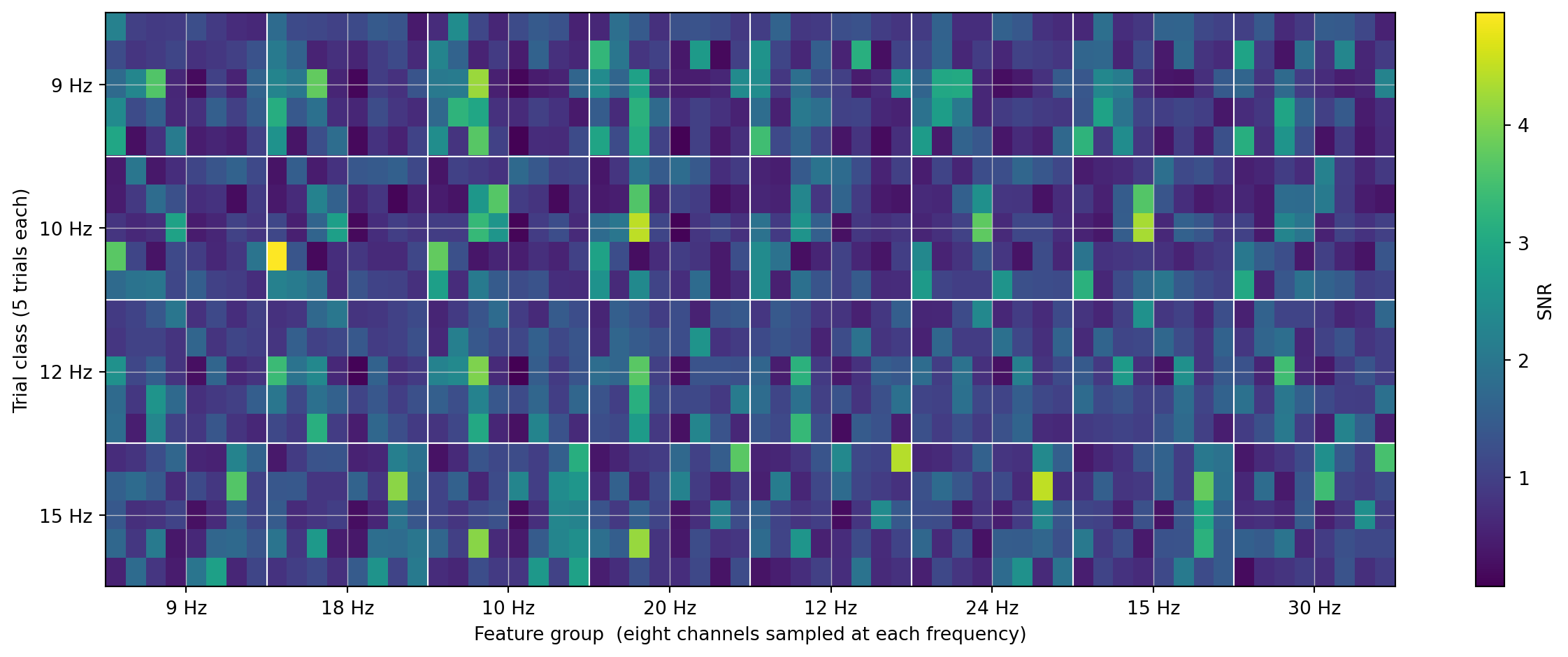
Figure 5.7: SNR feature matrix — same layout, but each cell is power at the target bin divided by mean power in adjacent bins.

The contrast sharpens. The brightest cells in each row are now even more concentrated in the column corresponding to that trial’s stimulation frequency, and the cross-class noise (especially in the 12/15 Hz blocks) drops away. SNR features are what we’ll feed to the classifier in Ch 7. The next chapter (Ch 6) develops a different family of features — template matching with CCA — that doesn’t need to commit to specific harmonics in advance.