4  Epoching: Recovering Trials from Triggers

The trial structure isn’t documented anywhere in the dataset. Reconstruct it from CH10, decide on epoch boundaries, and produce a tidy (trials × channels × time) array that every later chapter will consume.

4.1 Loading and filtering

Same setup as Ch 3 — running example, filter chain applied to all eight EEG channels. CH10 (the trigger) and CH11 (the LDA output) are integer step functions; filtering would smear them, so we leave them alone.

from pathlib import Path
import numpy as np
import scipy.io
import matplotlib.pyplot as plt
from scipy.signal import butter, filtfilt, iirnotch

DATA_DIR = Path("data")
EEG_LABELS = ["PO7", "PO3", "POz", "PO4", "PO8", "O1", "Oz", "O2"]

mat = scipy.io.loadmat(DATA_DIR / "subject_2_fvep_led_training_2.mat")
fs = int(mat["fs"][0, 0])
y = mat["y"]


def make_filters(fs, low=5.0, high=40.0, line=50.0, order=4, notch_q=30):
    bp_b, bp_a = butter(order, [low, high], btype="band", fs=fs)
    n_b, n_a = iirnotch(line, notch_q, fs=fs)
    return (bp_b, bp_a), (n_b, n_a)


def apply_filters(x, bp, notch):
    return filtfilt(*notch, filtfilt(*bp, x))


bp, notch = make_filters(fs)
y_filt = y.astype(float).copy()
for ci in range(1, 9):
    y_filt[ci] = apply_filters(y[ci], bp, notch)

print(f"y shape:      {y.shape}")
print(f"y_filt shape: {y_filt.shape}  (CH2–9 filtered, CH1/CH10/CH11 untouched)")

y shape:      (11, 57697)
y_filt shape: (11, 57697)  (CH2–9 filtered, CH1/CH10/CH11 untouched)

4.2 The trigger channel over time

ch10 = y[9].astype(int)
t = np.arange(len(ch10)) / fs

fig, ax = plt.subplots(figsize=(12, 3))
ax.plot(t, ch10, drawstyle="steps-post", lw=0.8)
ax.set_yticks([0, 9, 10, 12, 15])
ax.set_xlabel("Time (s)")
ax.set_ylabel("CH10 (Hz)")
ax.set_title("Trigger channel — full session")
fig.tight_layout()
fig.savefig("images/04-epoching_trigger_timeline.png", dpi=200, bbox_inches="tight")
plt.show()

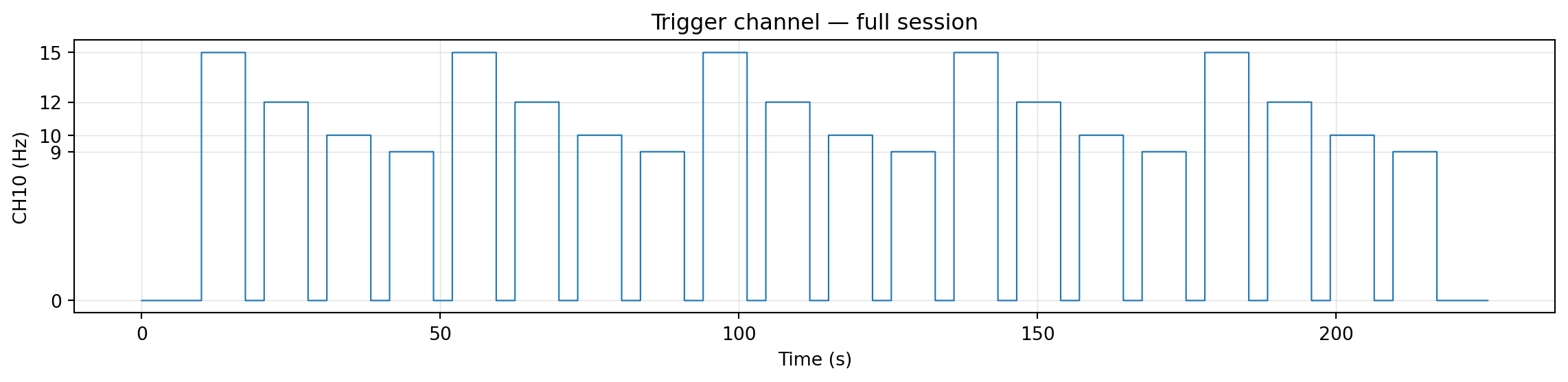
Figure 4.1: CH10 across the full session — the only document of trial structure we have.

A clean step function. CH10 sits at zero between trials and steps to one of {9, 10, 12, 15} while a stimulation block is active. The plateaus look identical in width and the rests between them look identical too — that’s the experimental schedule, hardcoded in g.tec’s stimulator. The class sequence cycles 15 → 12 → 10 → 9 and repeats five times. None of this is documented in data_description.txt; everything we know about trial timing comes from staring at this one channel.

4.3 Detecting trial boundaries

def find_trials(y):
    """Return [(start_idx, end_idx, freq_hz), ...] from CH10 transitions."""
    ch10 = y[9].astype(int)
    active = (ch10 != 0).astype(int)
    diff = np.diff(active)
    starts = np.where(diff == 1)[0] + 1
    ends = np.where(diff == -1)[0] + 1
    return [(int(s), int(e), int(ch10[s])) for s, e in zip(starts, ends)]


trials = find_trials(y)
durations = sorted({round((e - s) / fs, 3) for s, e, _ in trials})
print(f"Trials detected: {len(trials)}")
print(f"Distinct durations (s): {durations}")
print(f"First five trials (start_s, end_s, duration_s, class):")
for s, e, fr in trials[:5]:
    print(f"  ({s / fs:6.2f}, {e / fs:6.2f}, {(e - s) / fs:5.2f}, {fr})")

Trials detected: 20
Distinct durations (s): [7.355]
First five trials (start_s, end_s, duration_s, class):
  ( 10.00,  17.36,  7.36, 15)
  ( 20.50,  27.86,  7.36, 12)
  ( 31.00,  38.36,  7.36, 10)
  ( 41.50,  48.86,  7.36, 9)
  ( 52.00,  59.36,  7.36, 15)

Edge detection on (CH10 != 0): rising edges mark trial onsets, falling edges mark offsets. Twenty trials, all exactly 7.36 s long. The fact that every trial is the same length is convenient — it lets us build a rectangular tensor without padding decisions.

4.4 Trials per class

classes = sorted({fr for _, _, fr in trials})
counts = [sum(1 for _, _, fr in trials if fr == c) for c in classes]

fig, ax = plt.subplots(figsize=(7, 3.5))
bars = ax.bar([str(c) for c in classes], counts, color=["C0", "C1", "C2", "C3"])
for bar, c in zip(bars, counts):
    ax.text(bar.get_x() + bar.get_width() / 2, c + 0.05, str(c), ha="center", fontsize=10)
ax.set_xlabel("Stimulation class (Hz)")
ax.set_ylabel("Trials")
ax.set_ylim(0, max(counts) + 1)
ax.set_title("Trials per class — running session")
fig.tight_layout()
fig.savefig("images/04-epoching_trial_counts.png", dpi=200, bbox_inches="tight")
plt.show()

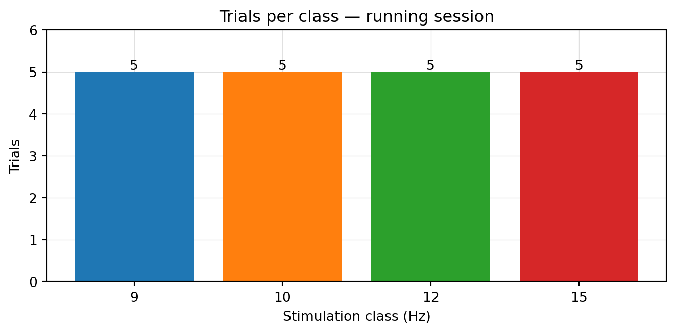
Figure 4.2: Trial count per stimulation class.

Five trials per class, perfectly balanced. Class balance matters for the classifier in Ch 7: an imbalanced training set biases the decision boundary toward the majority class. Five is a small training set per class — for now it’s what we have, and we’ll lean on cross-validation rather than a held-out split when we actually fit a model.

4.5 Building the epoch tensor

def epoch(y_filt, trials, eeg_idx=slice(1, 9)):
    """Stack trials into (n_trials, n_channels, n_samples). All trials must share length."""
    lengths = {e - s for s, e, _ in trials}
    if len(lengths) != 1:
        raise ValueError(f"Trials have varying lengths: {lengths}")
    n_samples = lengths.pop()
    epochs = np.stack([y_filt[eeg_idx, s:s + n_samples] for s, _, _ in trials])
    labels = np.array([fr for _, _, fr in trials])
    return epochs, labels


epochs, labels = epoch(y_filt, trials)
print(f"epochs shape: {epochs.shape}  (n_trials, n_channels, n_samples)")
print(f"labels shape: {labels.shape}, unique: {sorted(set(labels))}")
print(f"Per-trial duration: {epochs.shape[2] / fs:.2f} s")

epochs shape: (20, 8, 1883)  (n_trials, n_channels, n_samples)
labels shape: (20,), unique: [np.int64(9), np.int64(10), np.int64(12), np.int64(15)]
Per-trial duration: 7.36 s

This is the artifact every later chapter consumes. epochs is (20, 8, 1884) — twenty trials × eight EEG channels × 1884 samples (≈7.36 s at 256 Hz). labels is (20,) with values in {9, 10, 12, 15}. Slicing this tensor is how features get computed (Ch 5), how train/test splits get made (Ch 7), and how truncated-window experiments get run (Ch 8).

ep = epochs[0]
ep_label = labels[0]
t = np.arange(ep.shape[1]) / fs

fig, axes = plt.subplots(8, 1, figsize=(12, 9), sharex=True)
for i, ax in enumerate(axes):
    ax.plot(t, ep[i], lw=0.5)
    ax.set_ylabel(EEG_LABELS[i], fontsize=9, rotation=0, ha="right", va="center")
    ax.set_ylim(-50, 50)
    ax.tick_params(labelsize=7)
axes[-1].set_xlabel("Time (s)")
fig.suptitle(f"epochs[0]: {ep_label} Hz, {ep.shape[1] / fs:.2f} s, filtered", fontsize=10)
fig.tight_layout()
fig.savefig("images/04-epoching_example_epoch.png", dpi=200, bbox_inches="tight")
plt.show()

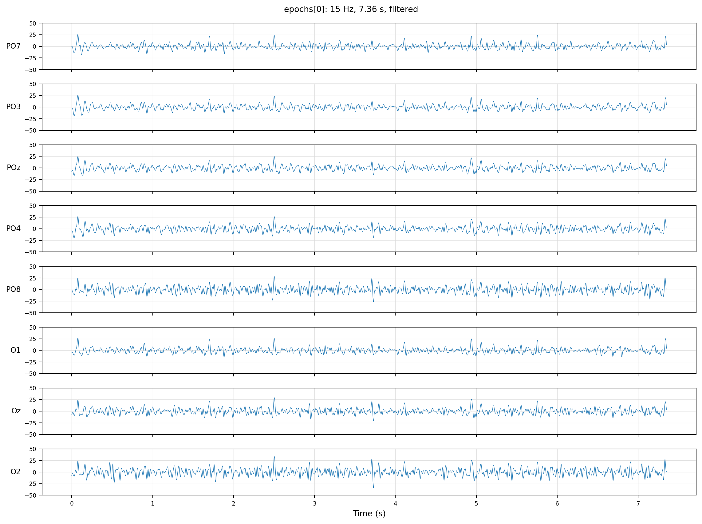
Figure 4.3: One epoch from the tensor — eight channels of the first trial, after filtering.

One trial, eight channels, the same shape that’s now stacked across all twenty. The slow baseline drift that wandered across the time-domain plots in Ch 3 is gone — this is what filtered, epoched data looks like, and from here on every chart will be built from epochs[i] slices.

4.6 Epoch length and the BCI tradeoff

We’ve used the full 7.36 s of each trial as the epoch length, which is generous. Longer epochs give more cycles of the SSVEP and so a more stable spectral estimate; they also mean the BCI has to wait longer before producing each decision. A real-time SSVEP keyboard typically operates on 1–4 s windows — short enough to feel responsive, long enough that the dominant peak is reliable. We come back to this in Ch 8 (time vs accuracy vs ITR), where we re-run the classifier on truncated epochs and trace out the tradeoff curve. For Ch 5 through Ch 7 we stay with the full-trial epoch as a baseline.