6  Template Features: CCA and FBCCA

A different way to score epochs against candidate frequencies: instead of reading bins from a spectrum, build sine/cosine reference templates at each candidate frequency and ask “how well does this epoch correlate with this template?” CCA finds the optimal channel mixture that maximizes that correlation, and FBCCA extends it across frequency sub-bands.

6.1 Setup: load, filter, epoch

Same pipeline as Ch 4 + 5; reproduced here so the chapter is self-contained.

from pathlib import Path
import numpy as np
import scipy.io
import matplotlib.pyplot as plt
from scipy.signal import butter, filtfilt, iirnotch
from sklearn.cross_decomposition import CCA

DATA_DIR = Path("data")
STIM_FREQS = [9, 10, 12, 15]
N_HARMONICS = 2

mat = scipy.io.loadmat(DATA_DIR / "subject_2_fvep_led_training_2.mat")
fs = int(mat["fs"][0, 0])
y = mat["y"]


def make_filters(fs, low=5.0, high=40.0, line=50.0, order=4, notch_q=30):
    bp_b, bp_a = butter(order, [low, high], btype="band", fs=fs)
    n_b, n_a = iirnotch(line, notch_q, fs=fs)
    return (bp_b, bp_a), (n_b, n_a)


def apply_filters(x, bp, notch):
    return filtfilt(*notch, filtfilt(*bp, x))


def find_trials(y):
    ch10 = y[9].astype(int)
    active = (ch10 != 0).astype(int)
    diff = np.diff(active)
    starts = np.where(diff == 1)[0] + 1
    ends = np.where(diff == -1)[0] + 1
    return [(int(s), int(e), int(ch10[s])) for s, e in zip(starts, ends)]


bp, notch = make_filters(fs)
y_filt = y.astype(float).copy()
for ci in range(1, 9):
    y_filt[ci] = apply_filters(y[ci], bp, notch)

trials = find_trials(y)
n_samples = trials[0][1] - trials[0][0]
epochs = np.stack([y_filt[1:9, s:s + n_samples] for s, _, _ in trials])
labels = np.array([fr for _, _, fr in trials])
print(f"epochs: {epochs.shape}, labels: {labels.shape}")

epochs: (20, 8, 1883), labels: (20,)

6.2 Reference templates

For each candidate stimulation frequency f, we build a synthetic reference signal — a small set of sines and cosines at f and its harmonics, sampled at the same length and rate as one epoch. CCA will then ask: which linear combination of the eight EEG channels correlates best with which linear combination of these reference signals?

def build_template(freq, n_samples, fs, n_harmonics=N_HARMONICS):
    """Return (n_samples, 2 * n_harmonics) array of sin/cos at freq, 2·freq, ..."""
    t = np.arange(n_samples) / fs
    refs = []
    for h in range(1, n_harmonics + 1):
        refs.append(np.sin(2 * np.pi * h * freq * t))
        refs.append(np.cos(2 * np.pi * h * freq * t))
    return np.stack(refs, axis=1)

template_9 = build_template(9, n_samples, fs)
t = np.arange(n_samples) / fs

fig, ax = plt.subplots(figsize=(11, 3))
labels_t = ["sin(2π·9·t)", "cos(2π·9·t)", "sin(2π·18·t)", "cos(2π·18·t)"]
for i, lab in enumerate(labels_t):
    ax.plot(t, template_9[:, i] - i * 2.5, lw=0.9, label=lab)
ax.set_xlim(0, 1)
ax.set_yticks([])
ax.set_xlabel("Time (s)")
ax.set_title("9 Hz template — first 1 s")
ax.legend(loc="upper right", ncol=4, fontsize=8)
fig.tight_layout()
fig.savefig("images/06-template-features_template.png", dpi=200, bbox_inches="tight")
plt.show()

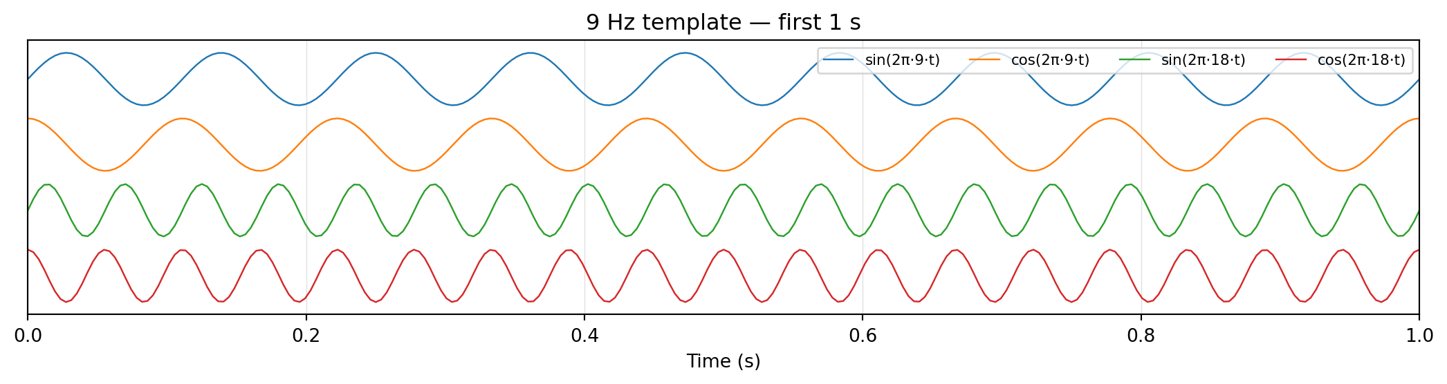
Figure 6.1: Reference template for the 9 Hz class — fundamental sin/cos plus second-harmonic sin/cos. First 1 second only, for legibility.

The template is deterministic — there’s no data here, just synthetic sines and cosines at 9 Hz and 18 Hz. CCA’s job is to find the best alignment between this template and the noisy 8-channel EEG; the strength of that alignment is the score for the “9 Hz” class. Including the harmonic in the template lets CCA pick up the same SSVEP information we sampled with the 2× features in Ch 5 — but here it’s done via correlation, which is sensitive to phase, not just power.

6.3 Scoring an epoch with CCA

Canonical correlation analysis finds the linear projection of the EEG channels and the linear projection of the template that are maximally correlated. We use only the largest canonical correlation (the first component) as the per-class score.

def cca_score(X, Y):
    """Largest canonical correlation between X (n_samples, n_x) and Y (n_samples, n_y)."""
    cca = CCA(n_components=1, max_iter=500)
    cca.fit(X, Y)
    Xc, Yc = cca.transform(X, Y)
    return float(np.corrcoef(Xc.ravel(), Yc.ravel())[0, 1])


def cca_class_scores(epoch, fs, freqs=STIM_FREQS, n_harmonics=N_HARMONICS):
    X = epoch.T  # (n_samples, n_channels)
    n_samples = X.shape[0]
    return np.array([cca_score(X, build_template(f, n_samples, fs, n_harmonics))
                     for f in freqs])

ti = 6
scores = cca_class_scores(epochs[ti], fs)
true_label = labels[ti]
colors = ["lightgray"] * 4
colors[STIM_FREQS.index(true_label)] = "C2"

fig, ax = plt.subplots(figsize=(7, 3.5))
bars = ax.bar([f"{f} Hz" for f in STIM_FREQS], scores, color=colors)
for bar, s in zip(bars, scores):
    ax.text(bar.get_x() + bar.get_width() / 2, s + 0.01, f"{s:.3f}", ha="center", fontsize=9)
ax.set_ylim(0, max(scores) * 1.15)
ax.set_ylabel("Canonical correlation")
ax.set_xlabel("Candidate class")
ax.set_title(f"Trial {ti} — true class is {true_label} Hz (green)")
fig.tight_layout()
fig.savefig("images/06-template-features_cca_scores.png", dpi=200, bbox_inches="tight")
plt.show()

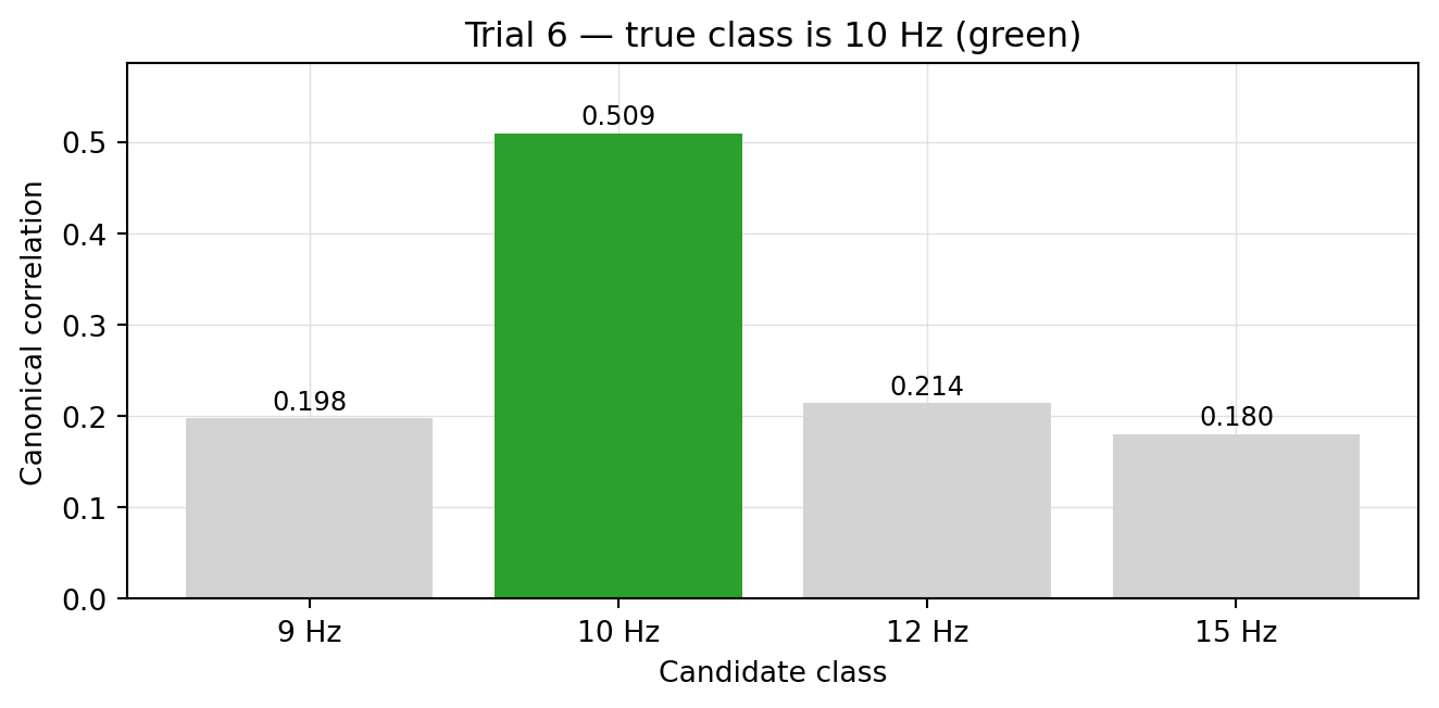
Figure 6.2: Per-class CCA scores for trial 6 — a 10 Hz trial. The true class wins by a comfortable margin.

The 10 Hz template wins (correlation ≈ 0.51) while the other three classes hover around 0.18–0.21. The decision rule is simple: pick the class whose template correlates most. No feature vector, no normalization, no neighborhood logic — just four scalars per trial.

6.4 All trials, all classes

score_mat = np.stack([cca_class_scores(ep, fs) for ep in epochs])
order = np.lexsort((np.arange(len(labels)), labels))
sorted_scores = score_mat[order]
sorted_labels = labels[order]

fig, ax = plt.subplots(figsize=(7, 6))
im = ax.imshow(sorted_scores, aspect="auto", origin="upper", cmap="viridis")
for r in np.where(np.diff(sorted_labels) != 0)[0] + 0.5:
    ax.axhline(r, color="white", lw=0.8)
ax.set_xticks(range(4))
ax.set_xticklabels([f"{f} Hz" for f in STIM_FREQS])
ax.set_xlabel("Candidate class")
yt = [np.where(sorted_labels == c)[0].mean() for c in sorted(set(sorted_labels))]
ax.set_yticks(yt)
ax.set_yticklabels([f"{c} Hz" for c in sorted(set(sorted_labels))])
ax.set_ylabel("Trial class (5 trials each)")
fig.colorbar(im, ax=ax, label="Canonical correlation")
fig.tight_layout()
fig.savefig("images/06-template-features_cca_matrix.png", dpi=200, bbox_inches="tight")
plt.show()

predictions = np.array([STIM_FREQS[i] for i in score_mat.argmax(axis=1)])
accuracy = (predictions == labels).mean()
n_correct = (predictions == labels).sum()
print(f"Plain CCA argmax accuracy: {n_correct}/{len(labels)} = {accuracy:.0%}")

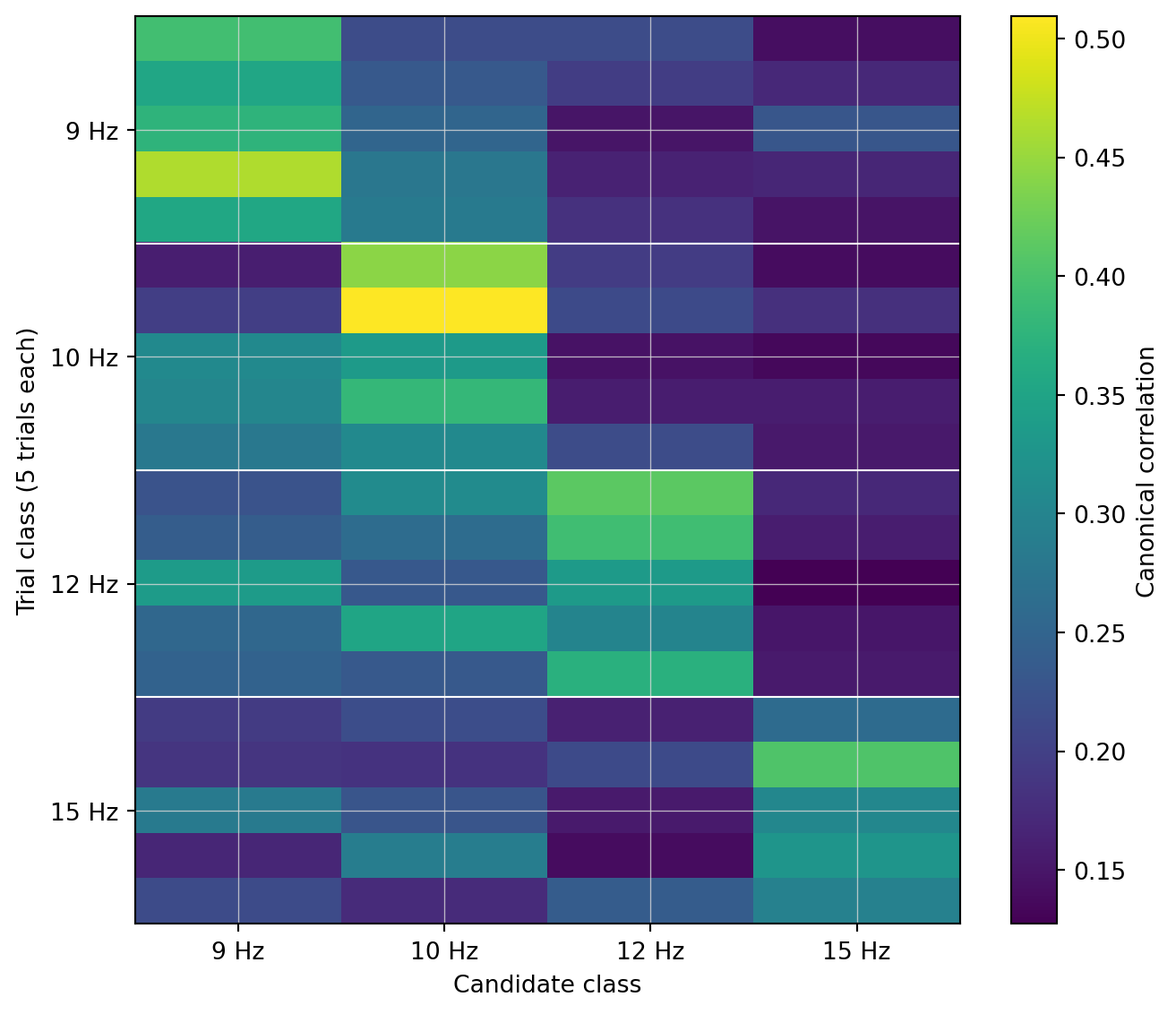
Figure 6.3: CCA scores for every (trial, candidate) pair. Rows are trials sorted by class. The brightest cell in each row should sit in the column matching that trial’s class.

Plain CCA argmax accuracy: 18/20 = 90%

90 % accuracy from a method that needed no training data. The two errors (visible in the heatmap as off-diagonal-block bright cells) are both 12 Hz trials confused with 9 or 10 Hz — the same alpha-overlap pattern we’ve been tracking since Ch 2. CCA partially handles alpha because it cares about the phase alignment between EEG and a 12 Hz template, not just the amount of 12 Hz power; but when alpha sits next to the stimulation frequency and the SSVEP response is weak, the alpha-driven channel mixture can correlate better with the wrong template.

6.5 Filter-bank CCA

The standard fix is FBCCA: split the filtered EEG into multiple sub-bands, run CCA per sub-band against the same templates, and combine the per-band correlations into a single score per class. Each sub-band isolates one harmonic family — the lowest band sees the fundamental, the next band sees the second harmonic, and so on — so CCA in each band can lock onto its target without being washed out by the others.

SUB_BANDS = [(6, 14), (14, 22), (22, 30), (30, 40)]
FBCCA_A, FBCCA_B = 1.25, 0.25  # Chen et al. 2015 weighting parameters


def fbcca_class_scores(epoch, fs, freqs=STIM_FREQS, sub_bands=SUB_BANDS,
                       a=FBCCA_A, b=FBCCA_B, n_harmonics=N_HARMONICS):
    n_samples = epoch.shape[1]
    weights = np.array([(i + 1) ** -a + b for i in range(len(sub_bands))])

    band_signals = []
    for low, high in sub_bands:
        b_, a_ = butter(4, [low, high], btype="band", fs=fs)
        band_signals.append(filtfilt(b_, a_, epoch, axis=-1))

    scores = np.zeros(len(freqs))
    for fi, freq in enumerate(freqs):
        Y = build_template(freq, n_samples, fs, n_harmonics)
        for bi, signal in enumerate(band_signals):
            r = cca_score(signal.T, Y)
            scores[fi] += weights[bi] * r ** 2
    return scores

ti = 9
cca_s = cca_class_scores(epochs[ti], fs)
fb_s = fbcca_class_scores(epochs[ti], fs)
true_label = labels[ti]

cca_n = cca_s / cca_s.max()
fb_n = fb_s / fb_s.max()
xpos = np.arange(len(STIM_FREQS))
w = 0.4

fig, ax = plt.subplots(figsize=(8, 3.8))
ax.bar(xpos - w / 2, cca_n, w, label="CCA", color="C0")
ax.bar(xpos + w / 2, fb_n, w, label="FBCCA", color="C1")
true_idx = STIM_FREQS.index(true_label)
ax.axvline(true_idx, color="C2", ls="--", alpha=0.6, label=f"true = {true_label} Hz")
ax.set_xticks(xpos)
ax.set_xticklabels([f"{f} Hz" for f in STIM_FREQS])
ax.set_ylabel("Score (normalized to max)")
ax.set_xlabel("Candidate class")
ax.set_title(f"Trial {ti} — CCA vs FBCCA")
ax.legend()
fig.tight_layout()
fig.savefig("images/06-template-features_fbcca.png", dpi=200, bbox_inches="tight")
plt.show()

print(f"Trial {ti} (true = {true_label} Hz):")
print(f"  CCA   scores: {dict(zip(STIM_FREQS, cca_s.round(3)))} → pick {STIM_FREQS[cca_s.argmax()]}")
print(f"  FBCCA scores: {dict(zip(STIM_FREQS, fb_s.round(3)))} → pick {STIM_FREQS[fb_s.argmax()]}")

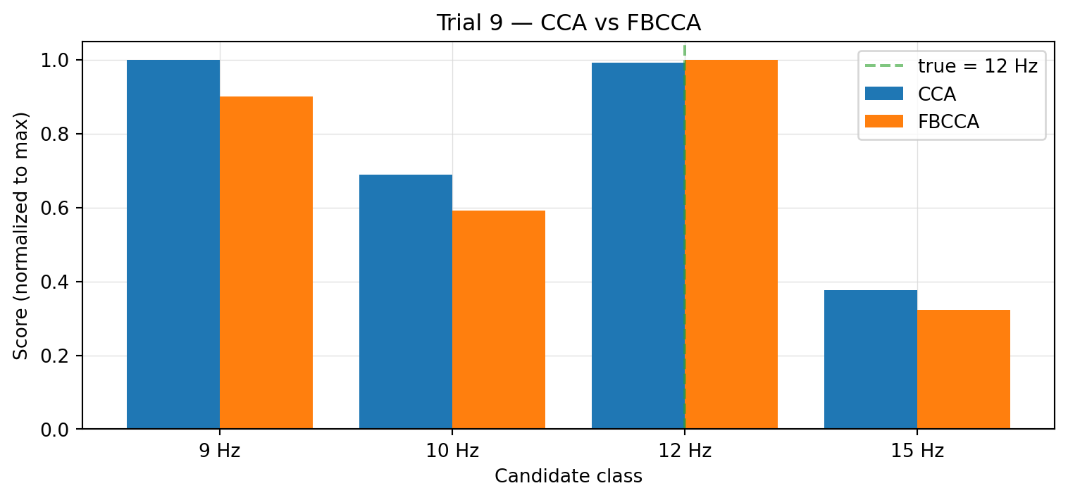
Figure 6.4: Per-class scores for one of the trials plain CCA gets wrong — trial 9 (true class: 12 Hz). Both methods are normalized to their own max for visual comparison. Plain CCA narrowly picks 9 Hz; FBCCA shifts the win to the correct 12 Hz.

Trial 9 (true = 12 Hz):
  CCA   scores: {9: np.float64(0.337), 10: np.float64(0.232), 12: np.float64(0.335), 15: np.float64(0.127)} → pick 9
  FBCCA scores: {9: np.float64(0.364), 10: np.float64(0.239), 12: np.float64(0.405), 15: np.float64(0.131)} → pick 12

fb_mat = np.stack([fbcca_class_scores(ep, fs) for ep in epochs])
fb_pred = np.array([STIM_FREQS[i] for i in fb_mat.argmax(axis=1)])
fb_acc = (fb_pred == labels).mean()
print(f"FBCCA argmax accuracy: {(fb_pred == labels).sum()}/{len(labels)} = {fb_acc:.0%}")

FBCCA argmax accuracy: 19/20 = 95%

FBCCA recovers one extra trial — 19/20 versus CCA’s 18/20 — at the cost of running CCA four times per epoch instead of once. The gain on this small session is modest (the alpha-vs-12-Hz collision is genuinely hard, and one of the two CCA errors persists), but the per-band weighting is tuneable, and on larger SSVEP datasets FBCCA typically pulls a few percentage points ahead. Ch 7 will show that even small score-gap improvements can translate into meaningful ITR (Ch 8) once we factor in trial duration.

The two methods give us our two main feature families: PSD-sampled features (Ch 5) — interpretable, easy to inspect — and template-correlation features (this chapter) — phase-aware, training-free per-trial scores. Both go into the classifier in the next chapter.