engram Cookbook

reference

quarto

The handbook for this repo - how it’s structured, the publishing workflow, and the Quarto authoring patterns I use, each shown as source + rendered output.

Published

June 16, 2026

Modified

June 25, 2026

How to use this cookbook

This is the living handbook for engram - a reference I keep coming back to and extend as I learn. It covers two things:

How the repo works - structure, conventions, and the render/publish workflow.
How to author a notebook - the Quarto features worth using.

For every visual feature in Part 2 you get two blocks: a Source block (the markup that produces it) and a Renders as block (what Quarto produces from it). Render locally with quarto preview to see the rendered halves live.

When you adopt something new, add a section and append a line to the Update log.

Note

A .ipynb carries Quarto front matter in a raw cell at the very top (the cell above this one). In a .qmd file the same YAML sits between --- fences.

Part 1 - The repo

Adding a new notebook

Drop the .ipynb into the relevant project folder (or create a new folder).
Add a front-matter raw cell at the top (see the starter).
Add a Colab badge as the first markdown cell.
Cite any papers with @key and add the entries to references.bib.
Run the notebook and save it with its outputs, then commit and push.

The notebook then appears automatically on the homepage listing - no manual index edit.

Render & publish workflow

The build never executes notebooks — it renders the outputs already saved in each .ipynb (execute: enabled: false in _quarto.yml). The runner needs no Python, no dependencies, and never downloads data.

So the rule is: run a notebook (locally or in Colab), save it with its outputs, then commit. A notebook committed without outputs renders with no figures.

quarto preview        # live preview while editing (renders saved outputs)
git add . && git commit -m "Add notebook" && git push

Pushing to main triggers the Action, which publishes to the gh-pages branch -> GitHub Pages at bkowshik.github.io/engram.

Part 2 - Authoring with Quarto

Each section below pairs the Source (what you write) with Renders as (what Quarto produces).

Front matter & metadata

Every notebook opens with a raw cell of YAML. This drives the title, the listing entry, categories, and per-document options. (The “rendered” effect here is the page’s title block and listing entry, not inline output.)

Source

---
title: 'Short, specific title'
description: 'One line - shown in the listing and the social card.'
date: '2026-06-16'
date-modified: last-modified # auto-updates from file mtime - good for living docs
categories: [eeg, pytorch, bci] # power the tag filter + listing
bibliography: references.bib # enables @citations
toc: true
code-tools: true # adds the "view source / copy" menu
image: thumbnail.png # optional - used in the social preview card
---

Callouts

Coloured boxes for asides, insights, and gotchas. Flavours: note, tip, warning, important, caution.

Source

::: {.callout-tip}

## Key insight

The takeaway in one or two sentences.
:::

::: {.callout-warning collapse="true"}

## Gotcha (collapsed by default)

Add `collapse="true"` to fold long asides.
:::

Renders as

Key insight

The takeaway in one or two sentences.

Gotcha (collapsed by default)

Add collapse="true" to fold long asides.

Math

Source

Inline: $h_t = \sigma(W x_t + b)$

$$
\mathcal{L} = \frac{1}{N}\sum_{i=1}^{N} -\,y_i \log \hat{y}_i
$$ {#eq-nll}

Reference it with `@eq-nll`.
$$

Renders as

Inline: $h_t = \sigma(W x_t + b)$

\[ \mathcal{L} = \frac{1}{N}\sum_{i=1}^{N} -\,y_i \log \hat{y}_i \tag{1}\]

The negative log-likelihood in Equation 1 is the loss the Shallow ConvNet trains with. $$

Citations & bibliography

With bibliography: references.bib in the front matter, cite inline and Quarto builds the reference list automatically.

Source

The Shallow ConvNet comes from @schirrmeister2017.
A parenthetical citation looks like [@schirrmeister2017].

…resolving against this .bib entry:

@article{schirrmeister2017,
  title   = {Deep learning with convolutional neural networks for EEG decoding and visualization},
  author  = {Schirrmeister, Robin Tibor and others},
  journal = {Human Brain Mapping}, year = {2017}, volume = {38}, pages = {5391--5420}
}

Renders as

The Shallow ConvNet comes from Schirrmeister et al. (2017). A parenthetical citation looks like (Schirrmeister et al. 2017). (The full reference appears in the auto-generated list at the end of the page.)

Diagrams (Mermaid & Graphviz)

Diagram-as-code - perfect for an architecture sketch instead of an ASCII block.

Source (4 outer backticks so the inner block shows literally)

```{mermaid}
flowchart LR
  X["EEG (22 ch x 1125)"] --> T["Temporal conv"]
  T --> S["Spatial conv"] --> P["Square -> pool -> log"] --> C["Classifier"]
```

Renders as

flowchart LR
  X["EEG (22 ch x 1125)"] --> T["Temporal conv"]
  T --> S["Spatial conv"] --> P["Square -> pool -> log"] --> C["Classifier"]

Code cells: source + output together

A code cell is the clearest case: by default Quarto shows both the source and the output it produces. The cell below is labelled and captioned so the figure can be cross-referenced - and its code stays visible above the plot.

Set %config InlineBackend.figure_format = "retina" once near the top so the saved plots are crisp on hi-DPI screens.

import numpy as np
import matplotlib.pyplot as plt
%config InlineBackend.figure_format = "retina"   # crisp hi-DPI plots

t = np.linspace(0, 1, 500)
x = np.sin(2 * np.pi * 10 * t)

plt.figure(figsize=(6, 2.4))
plt.plot(t, x)
plt.xlabel("Time (s)"); plt.ylabel("Amplitude")
plt.tight_layout()
plt.show()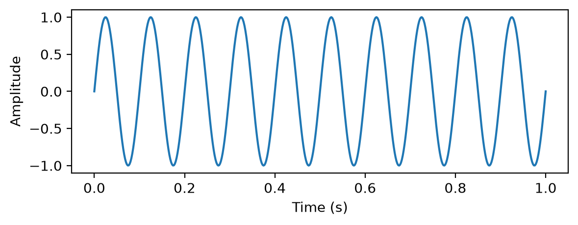

Figure 1: A 10 Hz sine wave - a stand-in for a band-limited neural signal.

Figure 1 shows the rendered output above, directly under the code that produced it. Control what each cell reveals with cell options:

Option	Effect
`# \| echo: false`	hide the code, keep the output
`# \| output: false`	run the code, hide the output
`# \| code-fold: true`	keep the code but collapse it behind a toggle
`# \| label: fig-x`/`tbl-x`	make it cross-referenceable (the `fig-`/`tbl-` prefix matters)
`# \| fig-cap: "..."`	figure caption
`# \| warning: false`	suppress warnings in the render

The default (echo: true) is exactly the “show both” behaviour - use the options above only when you deliberately want to hide one half.

Cross-references

Source

See @fig-signal and @eq-nll. Sections work too: tag a heading `{#sec-setup}`, then `@sec-setup`.

Renders as

See Figure 1 and Equation 1. Quarto numbers and links them automatically, so references never go stale when you reorder.

Tabsets

Stack alternatives behind tabs - handy for “same idea, two frameworks”.

Source

::: {.panel-tabset}

## NumPy

```python
import numpy as np
x = np.zeros((22, 1125))
```

## PyTorch

```python
import torch
x = torch.zeros(22, 1125)
```

:::

Renders as

import numpy as np
x = np.zeros((22, 1125))

import torch
x = torch.zeros(22, 1125)

Figures, captions & lightbox

Source

![Shallow ConvNet, Figure 2 from the paper.](architecture.png){#fig-arch}

Enable click-to-zoom for all images via _quarto.yml:

format:
  html:
    lightbox: true

Renders as: a captioned, numbered figure (Figure 1: ...) that is cross-referenceable with @fig-arch and opens in a zoom overlay on click.

Listings, categories & search (site-level)

These live in _quarto.yml / index.qmd, but every notebook feeds them:

Listing - index.qmd auto-indexes every **/*.ipynb, sorted by date.
Categories - the categories: in each notebook become clickable filters.
Full-text search - on by default; searches every notebook, client-side, free on GitHub Pages.

Social cards, comments & formats (site-level config)

These are _quarto.yml settings rather than inline output:

website:
  open-graph: true # rich link previews when shared
  twitter-card: true
  comments:
    giscus: # discussion thread per post, backed by GitHub Discussions
      repo: bkowshik/engram

format:
  html: default
  revealjs: # a speaker deck from the same notebook cells
    slide-level: 2

Render a slide deck from any notebook with quarto render notebook.ipynb --to revealjs.

No execution on build

engram sets this in _quarto.yml:

execute:
  enabled: false # render saved notebook outputs; never launch a kernel

This keeps publishing trivial: do the heavy compute wherever suits you (Colab, a GPU box, locally), save the notebook with its outputs, and the build just renders those - no kernel, no dependencies, no dataset downloads on CI.

If you would rather have the build execute notebooks and cache the results, the alternative is execute: freeze: auto plus a committed _freeze/ directory - but that needs the full environment available at render time.

Colab badge

Source (first markdown cell of a notebook)

[![Open In Colab](https://colab.research.google.com/assets/colab-badge.svg)](https://colab.research.google.com/github/bkowshik/engram/blob/main/FOLDER/NOTEBOOK.ipynb)

Renders as: a clickable “Open In Colab” badge that launches the notebook in Google Colab.

Copy-paste starter

Front matter for a new notebook (raw cell at the top):

---
title: ''
description: ''
date: 'YYYY-MM-DD'
date-modified: last-modified
categories: []
bibliography: references.bib
toc: true
code-tools: true
---

Before you push:

Front matter filled in (title, description, date, categories)
Colab badge points at the right folder/filename
Papers cited with @key, entries added to references.bib
Cells reveal what you intend (echo/output/code-fold)
Notebook saved with its outputs (the build never executes it)
Plots are retina (%config InlineBackend.figure_format = "retina")
No private references (paths, personal notes)

Update log

Append a line whenever you learn or adopt something new.

Date	Change
2026-06-16	Created. Each Part 2 feature now shows Source + Renders-as; example plot cell shows code and output together.

References

Schirrmeister, Robin Tibor, Jost Tobias Springenberg, Lukas Dominique Josef Fiederer, et al. 2017. “Deep Learning with Convolutional Neural Networks for EEG Decoding and Visualization.” Human Brain Mapping 38 (11): 5391–420. https://doi.org/10.1002/hbm.23730.